A radial filament in argon

A high-power beam can focus itself: the Kerr response raises the refractive index most strongly where the intensity is highest. Diffraction opposes that focusing. Above a characteristic critical power, the competition can drive a rapid rise in intensity. Photoionisation then creates free electrons whose response defocuses the beam and removes energy. A narrow high-intensity channel may persist over a substantial distance; this is optical filamentation.

We follow an initially collimated 800 nm pulse in argon at 1 bar. Its intensity FWHM is 30 fs, its 1/e² intensity radius is 300 μm, and its peak field on axis is \(1.21\times10^{10}\) V/m, which puts its peak power at three times the critical power returned by solprop’s Kerr model. Unlike a modal guide, the transverse profile is free to evolve. Cylindrical symmetry lets us resolve that evolution with one radial coordinate.

This lesson introduces the relation between fluence (energy per unit area), intensity (power per unit area), and electron density. The 128-point radial calculation shows developed focusing and plasma formation, but is not a converged prediction of a filament’s finest structure. It cannot describe azimuthal breakup or multiple off-axis filaments. See The free-space model and Envelope plasma: model, derivation and limits for the governing equations and assumptions.

Describe the beam and material

critical_power uses the Townes threshold for the cubic paraxial model, as a physical power in the medium at its carrier index. Setting the pulse above that threshold is a useful organising parameter, not a guarantee of a particular focus position in a broadband, ionising calculation. The beam is stated by its physical field: a Gaussian of 1/e² intensity radius WAIST (a radius, not a diameter or an intensity FWHM) times a temporal envelope of unit peak, scaled to FIELD and Hankel transformed. Its power and energy are then measured, in the argon, as the axial Poynting flux (Energy and flux in a medium). A SpatialPulse would fix the energy or the power instead.

import time

import matplotlib.pyplot as plt
import numpy as np

from solprop.boundaries import absorber
from solprop.constants import C
from solprop.driver import Simulation, SimulationSettings
from solprop.grid import EnvelopeGrid, RadialGrid
from solprop.nonlinear.envelope_plasma import EnvelopePlasmaResponse
from solprop.nonlinear.optmat_rates import OptmatRate
from solprop.nonlinear.responses import KerrResponse
from solprop.physdata import chi3, gamma3, refractive_index
from solprop.pulses import GaussianPulse
from solprop.spatial import (
    SpatialFlux,
    SpatialMedium,
    critical_power,
    spatial_energy,
    spatial_fluence,
    spatial_power,
)
from solprop.stats import StatsSpec
from solprop.stepper import PIController

Choose the grids and responses

The beam, the medium and the grids. The radial grid reaches four waists, so the light initially lies well inside the domain; check outward-moving light against the boundary when extending the run. The absorber makes its outer tenth an absorbing collar. The envelope plasma needs the range of field amplitudes its rate table must cover, here up to 1e11 V/m, well above the clamped field.

started = time.perf_counter()

WAIST = 300e-6
FIELD = 1.2127e10  # V/m, the peak of the analytic field on axis
LENGTH = 0.25
medium = SpatialMedium("Ar", pressure=1.0)
index = float(refractive_index("Ar", 2 * np.pi * C / 800e-9, pressure=1.0))
power = critical_power(800e-9, chi3("Ar", pressure=1.0, wavelength=800e-9), index=index)

grid = EnvelopeGrid.from_limits(LENGTH, 800e-9, (500e-9, 1.4e-6), 300e-15, thg=False)
space = RadialGrid(4 * WAIST, 128)
envelope = GaussianPulse(wavelength=800e-9, fwhm=30e-15, peak_power=1.0).build(grid)
profile = np.exp(-((space.r / WAIST) ** 2))
pulse = FIELD * space.hankel.forward(profile)[:, None, None] * envelope
flux = SpatialFlux.resolve(grid, space, medium)
peak_power = float(np.max(spatial_power(pulse, flux)))
responses = [
    KerrResponse(gamma3("Ar", wavelength=800e-9), thg=False),
    EnvelopePlasmaResponse("Ar", OptmatRate("Ar", 800e-9)),
]
settings = SimulationSettings(
    controller=PIController(rtol=1e-5, atol=1e-11),
    save_planes=np.linspace(0, LENGTH, 81)[1:],
    dz_init=1e-5,
    dz_max=5e-4,
    stats=StatsSpec(names=("energy", "peak_intensity", "electron_density")),
    absorber=absorber(grid),
    ionisation_field_range=(1e8, 1e11),
)
simulation = Simulation.from_radial(
    grid, space, medium, responses, pulse, settings=settings
)
run = simulation.run(progress="none")

Compare characteristic scales

Marburger’s empirical collapse distance for a collimated Gaussian, a comparison only: it describes a monochromatic paraxial beam in a pure Kerr medium, and nothing here depends on it. The coefficient and its scope are discussed with the references in The free-space model; plasma arrests the Kerr-only collapse, so the estimate is a reference marker rather than an expected answer.

ratio = peak_power / power
rayleigh = np.pi * index * WAIST**2 / 800e-9
marburger = 0.367 * rayleigh / np.sqrt((np.sqrt(ratio) - 0.852) ** 2 - 0.0219)
energy = np.asarray(run["stats/energy"]).reshape(-1)
print(f"critical power: {power * 1e-9:.4g} GW; beam: {peak_power * 1e-9:.4g} GW")
print(f"P/Pcr = {ratio:.4f}; launch energy {spatial_energy(pulse, flux) * 1e3:.4g} mJ")
print(f"pulse energy: {energy[0] * 1e3:.4g} mJ; Marburger distance: {marburger:.3g} m")

critical power: 9.2 GW; beam: 27.6 GW
P/Pcr = 3.0002; launch energy 0.8814 mJ
pulse energy: 0.8814 mJ; Marburger distance: 0.15 m

Read fluence and plasma together

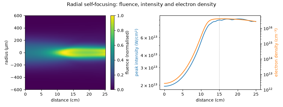
The fluence along the propagation, mirrored about the axis, and the peak intensity and electron density. The beam contracts slowly and collapses at about 11 cm, a little before Marburger’s estimate for a monochromatic beam (dotted). From there the intensity is clamped just below 10^14 W/cm^2 while the plasma is created: the filament is the bright channel, some 100 μm across, and the light the plasma defocuses forms the dimmer reservoir around it.

z = np.asarray(run["z"])
planes = run.planes()
# The medium is uniform, so one measure serves every plane.
fluence = np.array([spatial_fluence(plane.field, flux) for plane in planes])
radius = np.asarray(space.r)
mirrored = np.concatenate([-radius[::-1], radius])
map_values = np.concatenate([fluence[:, ::-1], fluence], axis=1)

figure, (left, right) = plt.subplots(1, 2, figsize=(9.5, 3.6))
figure.suptitle("Radial self-focusing: fluence, intensity and electron density")
image = left.pcolormesh(
    z * 1e2, mirrored * 1e6, map_values.T / map_values.max(), shading="auto"
)
left.set_ylim(-600, 600)
left.set_xlabel("distance (cm)")
left.set_ylabel("radius (μm)")
figure.colorbar(image, ax=left, label="fluence (normalised)")

intensity = np.asarray(run["stats/peak_intensity"]).reshape(-1)
electrons = np.asarray(run["stats/electron_density"]).reshape(-1)
right.plot(z * 1e2, intensity * 1e-4, color="C0")
right.set_xlabel("distance (cm)")
right.set_ylabel("peak intensity (W/cm²)", color="C0")
right.set_yscale("log")
twin = right.twinx()
twin.plot(z * 1e2, electrons * 1e-6, color="C1")
twin.set_ylabel("electron density (cm⁻³)", color="C1")
twin.set_yscale("log")
twin.set_ylim(bottom=1e12)
right.axvline(marburger * 1e2, color="0.6", ls=":", lw=1)
figure.tight_layout()

What the figures do and do not show

The left panel integrates the axial flux over the whole pulse. A bright fluence core therefore does not by itself tell us either the peak intensity or the duration. The right panel supplies the peak intensity and electron density: compare their rise with the contraction in the map. The signed radial axis is a mirrored view of one cylindrically symmetric solution, not two independently resolved sides.

Refine the radial samples, time window and wavelength band, and move the outer boundary before treating a peak intensity or plasma density quantitatively. Tightening the integration tolerance alone cannot repair unresolved spatial structure. Loss of energy can include ionisation and absorbing boundaries; check their contributions before attributing all loss to the gas.

The next lesson, Two crossing beams in Cartesian free space, removes radial symmetry to follow two crossing beams. For nonlinear free-space examples and the spatial transforms, continue with Free space: beams in bulk media and Radial Hankel transform.

print(f"exit energy / input energy: {energy[-1] / energy[0]:.6f}")
print(f"{time.perf_counter() - started:.1f} s; backend {run.metadata.backend.name}")

exit energy / input energy: 0.919088
35.3 s; backend numba_cpu