Supercontinuum by self-phase modulation#

A supercontinuum is a spectrum broadened by nonlinear propagation over an octave or more. How it is broadened decides its noise and coherence: whether every laser shot produces the same spectrum with the same spectral phase, which is what a pulse compressor or a frequency comb needs, or a spectrum that fluctuates from shot to shot because it grew from quantum noise.

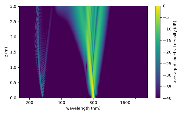
In this example self-phase modulation (SPM) in normal dispersion writes a mostly deterministic chirp onto the pulse. Spectral broadening can retain high coherence in this regime; the ensemble below checks that behaviour for this particular pulse, model and input-noise prescription. This example drives a long, large-core capillary filled with argon in a pressure gradient rising from vacuum at the entrance to 0.3 bar at the exit – the entrance is held at low pressure so that the high-energy pulse does not ionise the gas and self-focus as it is launched – with a 40 fs, 2 mJ pulse at 800 nm: a 3 m capillary of 225 um core radius, the regime of millijoule-level post-compression.

The ensemble: twenty shots of the same run with different realisations of the input shot noise. From them the example computes the averaged spectrum along the fibre, the relative intensity noise (RIN) of the exit spectrum – the shot-to-shot fluctuation of the spectral density – and its first-order coherence.

What to look for. The spectrum broadens smoothly and steadily towards the exit as the pressure rises; the RIN stays small and the coherence close to one across the whole continuum, down to its faint edges.

What is approximate. Only the fundamental mode is carried. Twenty shots provide a finite ensemble estimate; the RIN at the faint edges is especially sensitive to sampling.

The parameter choices follow panel (a) of the supercontinuum figure in the review by Travers et al.; these are regenerated solprop calculations, not the original figure data. The twenty seeded shots sample input optical noise only. They omit technical fluctuations of pulse energy, duration, coupling and gas pressure; convergence of ensemble statistics must be checked for the observable and spectral band of interest.

The ensemble#

Each shot is the same run with a different realisation of the quantum shot noise: one photon per active frequency bin and channel, with a random phase, added to the input spectrum (noise="input"), drawn from the generator seeded by seed.

import time
import warnings

import matplotlib.pyplot as plt
import numpy as np

from solprop.constants import C
from solprop.driver import prop_capillary
from solprop.exceptions import MaterialRangeWarning
from solprop.processing import g12_of, get_spectral_density

SHOTS = 20
"""The size of the ensemble."""

started = time.perf_counter()
runs = []
with warnings.catch_warnings():
    warnings.simplefilter("ignore", MaterialRangeWarning)
    for seed in range(SHOTS):
        runs.append(
            prop_capillary(
                225e-6,
                3.0,
                "Ar",
                (0.0, 0.3),
                lambda0=800e-9,
                fwhm=40e-15,
                energy=2e-3,
                trange=1e-12,
                wavelength_limits=(160e-9, 4e-6),
                noise="input",
                seed=seed,
                n_save=101,
                progress="none",
            )
        )

The averaged spectrum along the fibre#

The spectral energy density averaged over the ensemble, in decibels below its peak.

z = np.asarray(runs[0]["z"])
spectra = []
for run in runs:
    wavelength, density = get_spectral_density(run, "wavelength")
    spectra.append(density)
spectra = np.asarray(spectra)  # (shots, planes, wavelengths)
mean = spectra.mean(axis=0)
shown = (wavelength > 160e-9) & (wavelength < 2.6e-6)
ticks = [200, 400, 800, 1600]  # nm, labelled in full on the log axis

fig, ax = plt.subplots(figsize=(6.4, 4.0))
image = ax.pcolormesh(
    wavelength[shown] * 1e9,
    z,
    10 * np.log10(np.maximum(mean[:, shown] / mean.max(), 1e-12)),
    vmin=-40,
    vmax=0,
    shading="auto",
)
ax.set_xscale("log")
ax.set_xticks(ticks, labels=[str(tick) for tick in ticks])
ax.tick_params(axis="x", which="minor", labelbottom=False)
ax.set_xlabel("wavelength (nm)")
ax.set_ylabel("z (m)")
fig.colorbar(image, ax=ax, label="averaged spectral density (dB)")
fig.tight_layout()

Noise and coherence at the exit#

From top to bottom: the exit spectra of every shot (grey) and their mean (black); the relative intensity noise, the standard deviation of the spectral density over its mean, shot to shot; and the first-order coherence \(|g_{12}^{(1)}(\lambda)|\) of the ensemble’s complex spectra (0 for independent fields, 1 for identical ones).

exit_mean = spectra[:, -1].mean(axis=0)
rin = spectra[:, -1].std(axis=0) / exit_mean
omega, coherence = g12_of(runs, plane=-1)
coherent_wavelength = 2 * np.pi * C / omega
significant = exit_mean > 1e-4 * exit_mean[shown].max()

fig, (top, middle, bottom) = plt.subplots(3, 1, figsize=(6.4, 7.5), sharex=True)
for shot in spectra[:, -1]:
    top.semilogy(wavelength[shown] * 1e9, shot[shown], color="0.75", linewidth=0.5)
top.semilogy(wavelength[shown] * 1e9, exit_mean[shown], color="k", linewidth=1.0)
top.set_ylim(1e-6 * exit_mean[shown].max(), 3 * exit_mean[shown].max())
top.set_ylabel("spectral density (J/m)")
keep = shown & significant
middle.semilogy(wavelength[keep] * 1e9, rin[keep], color="tab:red", linewidth=1.0)
middle.set_ylabel("RIN")
in_window = (coherent_wavelength > 160e-9) & (coherent_wavelength < 2.6e-6)
bottom.plot(
    coherent_wavelength[in_window] * 1e9, coherence[in_window], color="tab:blue"
)
bottom.set_ylim(0, 1.05)
bottom.set_ylabel("coherence $|g_{12}|$")
bottom.set_xscale("log")
bottom.set_xticks(ticks, labels=[str(tick) for tick in ticks])
bottom.tick_params(axis="x", which="minor", labelbottom=False)
bottom.set_xlabel("wavelength (nm)")
fig.tight_layout()

weights = exit_mean[shown] / exit_mean[shown].sum()
mean_rin = float(np.sum(weights * np.nan_to_num(rin[shown])))
on_grid = np.interp(wavelength[shown], coherent_wavelength[::-1], coherence[::-1])
mean_coherence = float(np.nansum(weights * on_grid))
print(
    f"{len(runs)} shots; spectrally weighted RIN {mean_rin:.3e}, "
    f"spectrally weighted coherence {mean_coherence:.12f}"
)

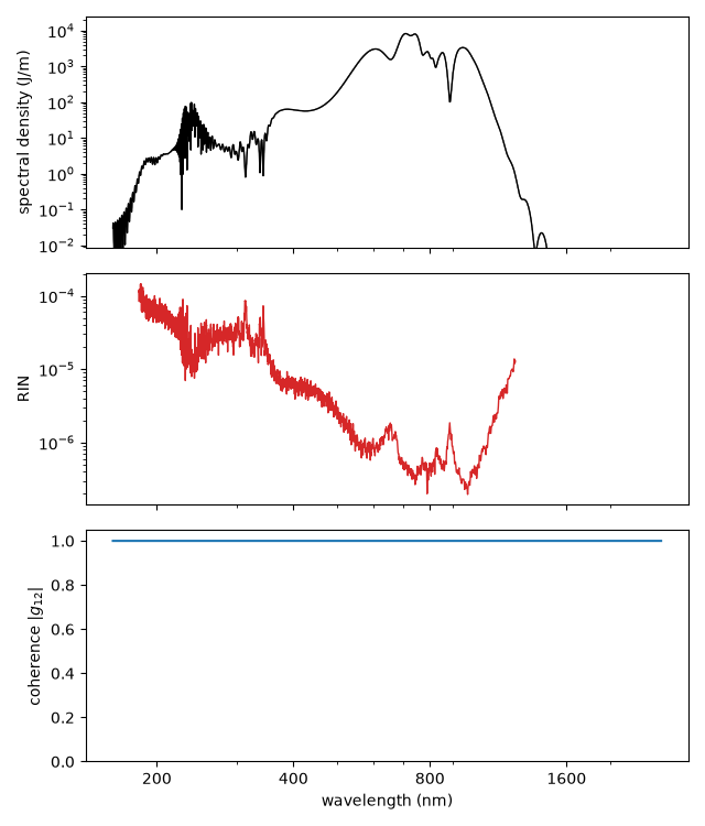
20 shots; spectrally weighted RIN 9.765e-07, spectrally weighted coherence 0.999999999993

Runtime and reproducibility#

print(
    f"{time.perf_counter() - started:.0f} s for {len(runs)} shots; "
    f"backend {runs[0].metadata.backend.name}"
)

153 s for 20 shots; backend native