Note
Go to the end to download the full example code.
Deep-ultraviolet four-wave mixing in argon under a frequency-dependent Kerr response#
A 400 nm pump and an 800 nm seed in an argon-filled capillary generate a deep-ultraviolet signal at 266.7 nm by degenerate four-wave mixing, \(\omega_s = 2\omega_p - \omega_i\), the phase-matched source of Durfee et al., Optics Letters 24, 697 (1999), doi:10.1364/OL.24.000697. The waveguide’s anomalous contribution to the dispersion cancels the gas’s normal one at one pressure, where \(2\beta(\omega_p) = \beta(\omega_i) + \beta(\omega_s)\).
The pump, seed and principal generated signal lie inside argon’s band edge (its two-photon resonance at a 189.4 nm fundamental), and their generating quartet lies above argon’s leg bound, 215.9 nm: the frequency-dependent responses of A frequency-dependent electronic response evaluate optmat’s fit itself here, for that quartet. Broadening and the full numerical band still need the material-region checks recorded by each run. So, unlike the helium dispersive wave, this comparison measures what the carrier approximation costs a phase-matched conversion. The coefficients that differ most from the carrier’s are not the generating quartet’s, 4 % above the pump’s Kerr value, but the signal’s cross-phase modulation by the pump, 25 % above it, and its own self-phase modulation, 57 % above it: phases, not gain.
The tutorial runs half a metre at the linear phase-matching pressure. This example adds what a design would ask next:
a metre of capillary, long enough for the signal to rise, saturate and fall back;
the pressure scan: the nonlinear phases detune the phase matching, so each response has its own best pressure, and the question is how much the carrier approximation misplaces it and misjudges the yield there;
pump depletion at each response’s best pressure, in photons.
What to look for. Every response converts best a little below the linear phase matching, and the dispersive responses about 10 mbar (5 %) lower than the carrier one, as their stronger cross-phase modulation of the signal by the pump requires. At the carrier policy’s best pressure it overstates the signal by about a tenth, and at the linear phase matching by a fifth; at each response’s own best pressure the yields agree to 2 %. The two dispersive evaluators agree to about a per cent throughout. At its best the signal carries a fifth of the pump’s photons, made from two fifths of them.
What is approximate. One mode, HE11, is carried; the radius and energies are this example’s choice, not Durfee et al.’s geometry. The argon index is optmat’s fit; its short-wavelength limit is 107.5 nm, below the active optical band of this example. Linear-index validity does not by itself qualify the electronic nonlinear response. Range warnings are suppressed in the setup below; inspect the material manifest when adapting it.
The frequency-dependent Kerr guide explains the response approximations. Use parameter scans when adapting the pressure search, and retain the band and material records.
The linear phase-matching pressure#
The zero of \(2\beta_p - \beta_i - \beta_s\) in the fundamental mode, formed from
neff - 1 so that the vacuum parts cancel exactly.
import math
import time
import warnings

import matplotlib.pyplot as plt
import numpy as np
from scipy.optimize import brentq

from solprop.constants import C
from solprop.driver import prop_capillary
from solprop.exceptions import MaterialRangeWarning
from solprop.modes import MarcatiliMode
from solprop.physdata import MaterialSelection
from solprop.processing import bandpass, energy, grid_of
from solprop.pulses import GaussianPulse

started = time.perf_counter()
POLICIES = ("carrier-kerr", "symmetric-kerr", "gas-polynomial")
COLOURS = {policy: f"C{index}" for index, policy in enumerate(POLICIES)}
RADIUS, LENGTH = 50e-6, 1.0
PUMP, IDLER = 400e-9, 800e-9
SIGNAL = 1.0 / (2.0 / PUMP - 1.0 / IDLER)
BANDS = {"signal": (250e-9, 285e-9), "pump": (340e-9, 480e-9)}
"""The signal's and the pump's bands, m: each holds its pulse and nothing else."""

omega = 2.0 * math.pi * C / np.array([PUMP, IDLER, SIGNAL])


def mismatch(pressure):
    """Return 2 beta_p - beta_i - beta_s of the HE_11 mode, 1/m."""
    excess = (
        omega / C * MarcatiliMode(RADIUS, "Ar", pressure).neff_minus_one(omega).real
    )
    return float(2.0 * excess[0] - excess[1] - excess[2])


with warnings.catch_warnings():
    warnings.simplefilter("ignore", MaterialRangeWarning)
    LINEAR = brentq(mismatch, 0.01, 5.0, xtol=1e-9)
print(f"signal {SIGNAL * 1e9:.1f} nm; linear phase matching at {LINEAR * 1e3:.1f} mbar")
signal 266.7 nm; linear phase matching at 209.4 mbar
The scan#
Each response over pressures around the linear phase matching, a metre of fibre, 10 uJ in each of a 30 fs pump and seed. Recorded for each run: the signal’s energy along the fibre and the pump’s.
def fwm_run(policy, pressure, n_save):
    """Propagate the argon case under one electronic policy at one pressure, bar."""
    with warnings.catch_warnings():
        # Range notices are suppressed for the setup; inspect the manifest when
        # changing the band.
        warnings.simplefilter("ignore", MaterialRangeWarning)
        return prop_capillary(
            RADIUS,
            LENGTH,
            "Ar",
            pressure,
            lambda0=PUMP,
            pulses=[
                GaussianPulse(wavelength=PUMP, fwhm=30e-15, energy=10e-6),
                GaussianPulse(wavelength=IDLER, fwhm=30e-15, energy=10e-6),
            ],
            wavelength_limits=(210e-9, 2e-6),
            trange=250e-15,
            n_save=n_save,
            materials=MaterialSelection(electronic=policy),
            progress="none",
        )


def band_energies(run):
    """Return each band's energy at every saved plane, J."""
    grid = grid_of(run)
    planes = np.asarray(run["z"]).size
    return {
        name: np.array(
            [
                float(np.sum(energy(run, plane=i, bandpass=bandpass(grid, band))))
                for i in range(planes)
            ]
        )
        for name, band in BANDS.items()
    }


pressures = LINEAR * np.linspace(0.7, 1.15, 19)
scan = {policy: [] for policy in POLICIES}
for policy in POLICIES:
    for pressure in pressures:
        signal = band_energies(fwm_run(policy, pressure, n_save=41))["signal"]
        scan[policy].append((signal.max(), signal[-1]))
scan = {policy: np.array(rows) for policy, rows in scan.items()}

fig, (left, right) = plt.subplots(1, 2, figsize=(10.0, 3.6), layout="constrained")
for policy in POLICIES:
    left.plot(
        1e3 * pressures,
        1e6 * scan[policy][:, 0],
        "o-",
        ms=3,
        color=COLOURS[policy],
        label=policy,
    )
    right.plot(
        1e3 * pressures,
        1e6 * scan[policy][:, 1],
        "o-",
        ms=3,
        color=COLOURS[policy],
        label=policy,
    )
for ax, title in ((left, "largest along the fibre"), (right, "at the exit of 1 m")):
    ax.axvline(1e3 * LINEAR, color="0.6", lw=0.8, ls="--")
    ax.set_xlabel("pressure (mbar)")
    ax.set_title(title)
left.set_ylabel("250-285 nm energy (uJ)")
left.legend(frameon=False)

print("pressure (mbar)   largest signal (uJ): " + "  ".join(POLICIES))
for index, pressure in enumerate(pressures):
    print(
        f"{1e3 * pressure:14.1f}   "
        + "  ".join(f"{1e6 * scan[policy][index, 0]:12.3f}" for policy in POLICIES)
    )

best = {}
for policy in POLICIES:
    index = int(np.argmax(scan[policy][:, 0]))
    best[policy] = pressures[index]
    print(
        f"{policy:15s} best {1e3 * pressures[index]:5.1f} mbar: largest signal "
        f"{1e6 * scan[policy][index, 0]:.2f} uJ; at the exit "
        f"{1e6 * scan[policy][index, 1]:.2f} uJ"
    )
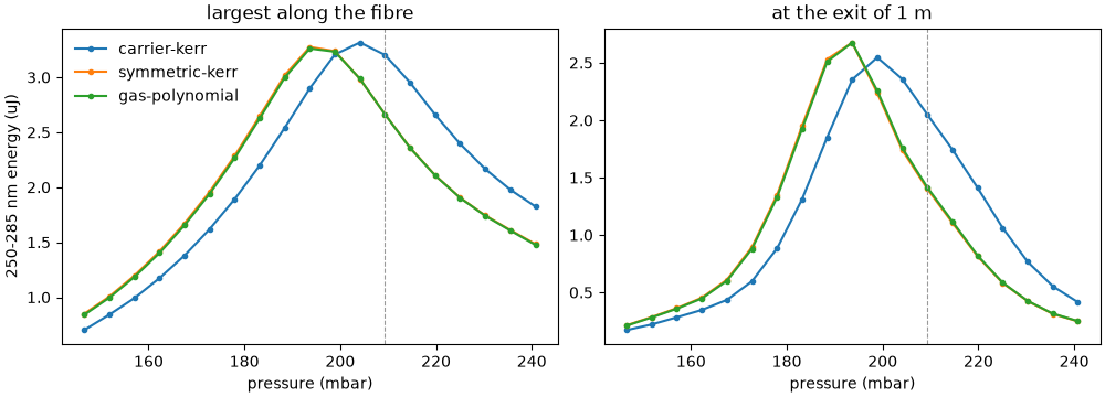
pressure (mbar)   largest signal (uJ): carrier-kerr  symmetric-kerr  gas-polynomial
         146.5          0.702         0.849         0.840
         151.8          0.842         1.006         0.995
         157.0          0.991         1.196         1.183
         162.3          1.173         1.415         1.402
         167.5          1.379         1.670         1.654
         172.7          1.618         1.957         1.939
         178.0          1.891         2.284         2.264
         183.2          2.198         2.647         2.625
         188.4          2.541         3.018         2.997
         193.7          2.900         3.275         3.261
         198.9          3.206         3.237         3.232
         204.1          3.316         2.985         2.986
         209.4          3.202         2.662         2.662
         214.6          2.952         2.359         2.357
         219.8          2.659         2.108         2.107
         225.1          2.394         1.904         1.902
         230.3          2.165         1.743         1.740
         235.5          1.977         1.611         1.606
         240.8          1.825         1.483         1.477
carrier-kerr    best 204.1 mbar: largest signal 3.32 uJ; at the exit 2.36 uJ
symmetric-kerr  best 193.7 mbar: largest signal 3.28 uJ; at the exit 2.68 uJ
gas-polynomial  best 193.7 mbar: largest signal 3.26 uJ; at the exit 2.68 uJ
The dashed line is the linear phase matching. Every response converts best a little below it, where the nonlinear phases are balanced by a waveguide contribution that is no longer cancelled by the gas; the dispersive responses, whose cross-phase modulation of the signal is a quarter stronger than the carrier’s, need about 10 mbar less. The scan’s step is 2.5 % of the linear pressure, which is how well each best pressure is known. The whole curve moves: at the carrier policy’s best pressure the dispersive responses give about a tenth less signal than it predicts, at the linear phase matching a fifth less, while each response’s best yield is the same to 2 %. The carrier approximation misplaces the operating point; it hardly misjudges what the best operating point delivers.
Pump depletion at each response’s best pressure#
The signal’s and the pump’s energies along the fibre, and the conversion in photons: the signal photons made per pump photon launched. Each signal photon costs two pump photons, so the conversion can at most reach one half.
fig, (left, right) = plt.subplots(1, 2, figsize=(10.0, 3.6), layout="constrained")
for policy in POLICIES:
    run = fwm_run(policy, best[policy], n_save=101)
    z = np.asarray(run["z"])
    bands = band_energies(run)
    photons = (bands["signal"] * SIGNAL) / (bands["pump"][0] * PUMP)
    left.plot(z, 1e6 * bands["signal"], lw=1.6, color=COLOURS[policy], label=policy)
    left.plot(z, 1e6 * bands["pump"], lw=1.0, ls="--", color=COLOURS[policy])
    right.plot(z, photons, lw=1.6, color=COLOURS[policy], label=policy)
    peak = int(np.argmax(bands["signal"]))
    print(
        f"{policy:15s} at {1e3 * best[policy]:5.1f} mbar: signal "
        f"{1e6 * bands['signal'][peak]:.2f} uJ at {z[peak]:.2f} m, "
        f"{photons[peak]:.2f} of the pump's photons; the pump there "
        f"{1e6 * bands['pump'][peak]:.2f} uJ of {1e6 * bands['pump'][0]:.2f}"
    )
left.set_xlabel("z (m)")
left.set_ylabel("energy (uJ): signal (solid), pump (dashed)")
left.legend(frameon=False)
right.set_xlabel("z (m)")
_ = right.set_ylabel("signal photons per launched pump photon")
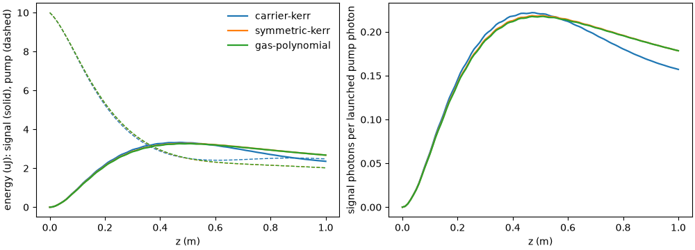
carrier-kerr    at 204.1 mbar: signal 3.33 uJ at 0.47 m, 0.22 of the pump's photons; the pump there 2.59 uJ of 10.00
symmetric-kerr  at 193.7 mbar: signal 3.28 uJ at 0.51 m, 0.22 of the pump's photons; the pump there 2.48 uJ of 10.00
gas-polynomial  at 193.7 mbar: signal 3.26 uJ at 0.51 m, 0.22 of the pump's photons; the pump there 2.49 uJ of 10.00
The signal turns over after about half a metre, when three quarters of the pump band’s energy has gone and a fifth of the pump’s photons have become signal photons, using two fifths of them; past that, the signal falls. The two dispersive evaluators – the polynomial exactly, the symmetric factorisation within 0.6 % on the quartets of the tutorial’s table – trace the same curves. The carrier approximation’s error in this case is not in the gain but in the phases: a design tuned with it would sit at the wrong pressure, and at that pressure expect more signal than the gas gives.
Runtime and reproducibility#
print(f"{time.perf_counter() - started:.0f} s; backend {run.metadata.backend.name}")
194 s; backend native
Total running time of the script: (3 minutes 13.816 seconds)