A pressure-gradient soliton compressor

A hollow capillary filled with a noble gas is the standard way to take a ten-femtosecond pulse at the few-hundred-microjoule level down to a single optical cycle. The pulse is launched in the anomalous-dispersion regime of the gas-filled guide, where self-phase modulation and anomalous dispersion together make it a higher-order soliton; it then self-compresses, reaching its shortest and most intense point at roughly the fission length, and at that point sheds a resonant dispersive wave in the deep ultraviolet.

The difficulty is getting the compressed pulse out. It exists only over a few centimetres, and a constant fill keeps working on it after it has formed: the pulse fissions, broadens and walks apart. A decreasing pressure gradient – the gas fed in at the entrance and pumped away at the exit – does two things at once. The nonlinearity falls towards the exit, so the compression slows and completes close to the end of the fibre, and the last centimetres are nearly evacuated, so the pulse experiences less material dispersion and nonlinearity near the exit. Waveguide dispersion remains even at zero gas density. This is the geometry of the few-femtosecond compressors of Travers et al., Nat. Photon. 13, 547 (2019) and Brahms et al., Phys. Rev. Research 2, 043037 (2020), here at a reduced size.

This example propagates it, with four HE_1m modes and the capillary’s coherent wall (Coherent capillary walls), and compares it with a constant fill of the same length. It then scans the entrance pressure to find the best compression, which is the question a design actually starts from.

What to look for. At this energy the pulse is a low-order soliton (the design tools below give \(N \approx 2.6\)), so it compresses cleanly from 10 fs to about 2 fs – below one optical cycle of the 800 nm carrier in the width of its power – and sheds almost nothing into the ultraviolet. The gradient compresses it earlier than a constant fill of the same mean density, because the density, and with it the nonlinearity, is highest where the pulse enters, and then holds it compressed through much of the low-density final section in this calculation. The pressure scan at the end shows how sharply the exit duration depends on the fill, and that at equal mean density the two fills reach much the same optimum: in this model the gradient’s advantage is not a shorter pulse but where the pulse is when it is shortest – at an evacuated exit, which in the laboratory needs no window and leaves no gas to disperse the pulse on its way out.

What is approximate. The gas’s refractive index is optmat’s fit, qualified over the whole band (helium’s from 60 nm); the gradient is the steady-state viscous-flow profile; the four retained modes leave only about a part in a thousand outside HE_11 in this case (printed below), but a small higher-mode population alone does not establish convergence with mode count; the wall is the outgoing Robin boundary condensed onto the retained modes, whose departure from Marcatili’s loss is a few parts in \(10^5\) for this bore.

The set-up

A 125 um core-radius capillary two metres long, filled with helium, pumped at 800 nm by a 10 fs, 250 uJ pulse. The window runs from 90 nm, far enough to hold the dispersive wave, to 3 um; the time window is 250 fs, which the compressed pulse and the wave emitted ahead of it both fit inside.

Before any propagation, the design tools say what regime this is. At the mean density estimated from an ideal viscous gradient from 0.8 bar to vacuum – two thirds of the entrance pressure in that approximation – the pulse is a soliton of order 2.6 with a fission length of 1.7 m, comparable to the fibre: it compresses once, strongly, and does not have room to fission.

import time
import warnings

import matplotlib.pyplot as plt
import numpy as np

from solprop.driver import prop_capillary
from solprop.exceptions import (
    GrazingIncidenceWarning,
    SolpropWarning,
)
from solprop.modes import CoherentWall
from solprop.plotting import prop_2d, time_1d
from solprop.processing import bandpass, energy, fwhm_t, get_power, grid_of
from solprop.processing import peak_power as peak_power_of
from solprop.tools import capillary_params

RADIUS = 125e-6
"""Core radius, m."""

LENGTH = 2.0
"""Capillary length, m."""

ENTRANCE = 0.8
"""Entrance pressure of the gradient, bar; the exit is evacuated."""

PUMP_BAND = (300e-9, 3e-6)
"""The band the compressed pulse is measured in, m.

The dispersive wave is emitted ahead of the pump and overlaps its leading edge; the
total power then beats at their difference frequency, which makes the width of the
*total* power a sub-femtosecond fringe rather than the pulse. Durations and peak
powers below are of the pump band alone, through a band-pass."""

PUMP = {"lambda0": 800e-9, "fwhm": 10e-15, "energy": 250e-6}
"""The pump: wavelength (m), duration (s) and energy (J)."""

UV = (100e-9, 250e-9)
"""The band the dispersive wave is counted in, m."""

started = time.perf_counter()

design = capillary_params(
    RADIUS,
    "He",
    2.0 * ENTRANCE / 3.0,
    energy=PUMP["energy"],
    fwhm=PUMP["fwhm"],
    wavelength=PUMP["lambda0"],
    shape="gauss",
)
print(design)

MODE:
  MarcatiliMode(HE11, a=125 um, He, model=full, loss=True)
WAVEGUIDE:
  Aeff = 2.34e-08 m^2, Lloss = 7.06e+00 m (1/e power)
FILL:
  0.533 bar He at 293.15 K, Pcr = 4.89e+11 W,
  gamma = 6.51e-11 /(W m), n2 = 1.94e-21 cm^2/W
PULSE:
  2.500e-04 J, 1.000e-14 s @ 800.0 nm (shape: gauss)
DISPERSION:
  -7.971e-30 s^2/m @ 800.0 nm, ZDW = 403.9 nm
POWER:
  2.35e+10 W (0.0480 of Pcr)
INTENSITY:
  1.00e+14 W/cm^2 mode-averaged, 1.78e+14 W/cm^2 on axis
SOLITON:
  Ld = 4.52e+00 m, Lnl = 6.54e-01 m, Lfiss = 1.72e+00 m, N = 2.63
CONSTITUENTS (unchirped NLSE):
  2 discrete solitons, area/pi = 2.1
  largest P = 6.006e+10 W, T = 1.428e-15 s, kNL = 1.955e+00 1/m

The propagation

One call per fill. modes=4 builds HE_11 to HE_14, which is the contiguous set the coherent wall needs; wall=CoherentWall() couples them through the capillary wall instead of giving each its own Marcatili loss. A pressure pair (p_in, p_out) is the steady-flow gradient. dz_max caps the step: a coupled flow needs one, because the interaction picture inverts the flow over a whole step and a half-metre step of a lossy four-mode block would amplify the source beyond what the flow admits (the refusal names this). Nothing else is chosen: Kerr, third-harmonic generation and photoionisation (optmat’s recommended rate for helium) are on by default, and the backend is the default "auto", which is the native build where one is installed.

def propagate(pressure):
    """Propagate the pump through the capillary at one fill."""
    with warnings.catch_warnings():
        # Two notices every run repeats, each one of the approximations named at
        # the top: the wall's quasi-static ratio comes within a factor ten of its
        # limit at the band's longest wavelengths; and the wall's generator is
        # resolved along z to the round-off floor of its samples, which it reports.
        for category in (GrazingIncidenceWarning, SolpropWarning):
            warnings.simplefilter("ignore", category)
        return prop_capillary(
            RADIUS,
            LENGTH,
            "He",
            pressure,
            wavelength_limits=(90e-9, 3e-6),
            trange=250e-15,
            modes=4,
            wall=CoherentWall(),
            dz_max=5e-3,
            n_save=201,
            progress="none",
            **PUMP,
        )


gradient = propagate((ENTRANCE, 0.0))
constant = propagate(2.0 * ENTRANCE / 3.0)
print(gradient)

MemoryOutput
  state:           closed
  planes:          201, 0 m to 2 m
  field per plane: 4 x 1 x 2049 (modes x components x omega)
  statistics:      core_radius, density, electron_density, energy, fwhm_t, fwhm_t_out...
  between planes:  none
  run:             RunMetadata(multimode, field grid of 4096, 4 modes, native, 2026-1...

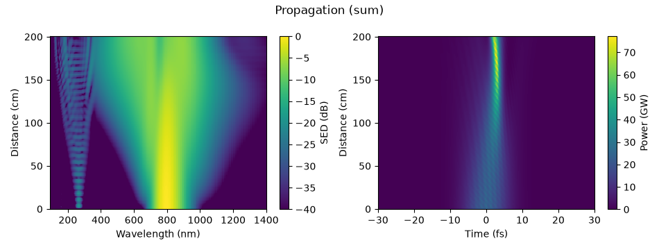
The gradient run, as a propagation map: the spectrum along the fibre on the left, in decibels below its peak and summed over the four modes, and the power in time on the right. The spectrum broadens steadily as the pulse compresses, reaching from 350 nm to 1.3 um. The faint fringed band near 267 nm from the entrance is the pump’s third harmonic, which the real-field Kerr term generates; it is strongest in the higher modes, where it is closer to phase matching, and it stays at the 1e-4 level.

figures = prop_2d(
    gradient,
    "wavelength",
    wavelength_range=(90e-9, 1.4e-6),
    trange=(-30e-15, 30e-15),
    db_min=-40,
    modes="sum",
)
figures[-1].set_size_inches(9.5, 3.6)
figures[-1].tight_layout()

Compression along the fibre

The peak power summed over the modes (peak_power(..., modes="sum"), the peak of the total power, not the largest single-mode peak) and the duration at each save plane, for both fills, measured in the pump band (bandpass=PUMP_BAND). The gradient reaches its shortest pulse about 20 cm before the exit and holds it; the constant fill is still compressing when the fibre ends. The ripple on the peak power is the beat between HE_11 and the small part of the pulse in the higher modes.

fig, (top, bottom) = plt.subplots(2, 1, figsize=(6.4, 5.2), sharex=True)
for run, name in (
    (gradient, f"{ENTRANCE} bar to vacuum"),
    (constant, f"constant {2.0 * ENTRANCE / 3.0:.2f} bar"),
):
    z = np.asarray(run["z"])
    top.plot(z, peak_power_of(run, modes="sum", bandpass=PUMP_BAND) * 1e-9, label=name)
    bottom.plot(z, fwhm_t(run, modes="sum", bandpass=PUMP_BAND) * 1e15, label=name)
top.set_ylabel("peak power (GW)")
bottom.set_ylabel("FWHM duration (fs)")
bottom.set_xlabel("z (m)")
bottom.set_ylim(0.0, 25.0)
top.legend(frameon=False)
fig.tight_layout()

for run, name in ((gradient, "gradient"), (constant, "constant")):
    power = peak_power_of(run, modes="sum", bandpass=PUMP_BAND)
    best = int(np.argmax(power))
    z = np.asarray(run["z"])
    print(
        f"{name:9s}: largest peak power {power[best] * 1e-9:.1f} GW at "
        f"z = {z[best]:.3f} m; at the exit {power[-1] * 1e-9:.1f} GW and "
        f"{fwhm_t(run, plane=-1, modes='sum', bandpass=PUMP_BAND) * 1e15:.2f} fs"
    )

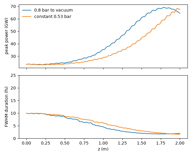
gradient : largest peak power 69.2 GW at z = 1.790 m; at the exit 64.4 GW and 2.02 fs
constant : largest peak power 68.4 GW at z = 1.970 m; at the exit 67.7 GW and 1.66 fs

The exit pulse

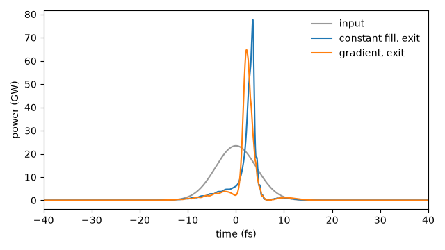
The power in time at the exit of each fibre, beside the input: both deliver a single dominant peak about 2 fs wide on a small pedestal, the pedestal being the part of the pulse self-phase modulation did not bring into phase.

fig, ax = plt.subplots(figsize=(6.4, 3.6))
t, power = get_power(gradient, plane=0, modes="sum", oversampling=8)
ax.plot(t * 1e15, power * 1e-9, color="0.6", label="input")
for run, name in ((constant, "constant fill, exit"), (gradient, "gradient, exit")):
    t, power = get_power(run, plane=-1, modes="sum", oversampling=8)
    ax.plot(t * 1e15, power * 1e-9, label=name)
ax.set_xlim(-40.0, 40.0)
ax.set_xlabel("time (fs)")
ax.set_ylabel("power (GW)")
ax.legend(frameon=False)
fig.tight_layout()

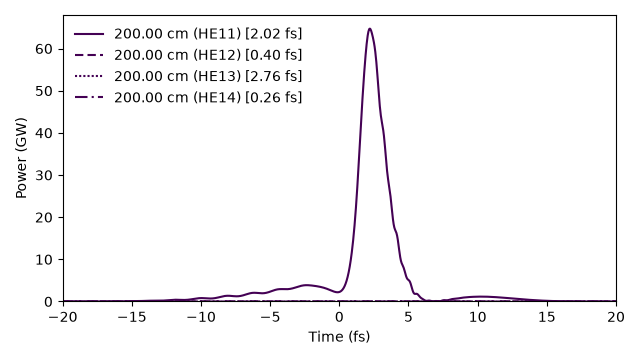
time_1d draws the same exit pulse for each mode, with its width marked: the compressed pulse is almost entirely in HE_11; the higher modes hold the part of it that the Kerr overlap between the modes moved there, three orders of magnitude weaker.

fig, ax = plt.subplots(figsize=(6.4, 3.6))
time_1d(gradient, trange=(-20e-15, 20e-15), ax=ax)
fig.tight_layout()

Where the energy went

The energy in each mode at the exit, and in the ultraviolet band. The ultraviolet is counted with a band-pass, solprop.processing.spectra.bandpass(), on the run’s own grid.

for run, name in ((gradient, "gradient"), (constant, "constant")):
    start = float(np.sum(energy(run, plane=0)))
    per_mode = np.asarray(energy(run, plane=-1)) / start
    uv = float(np.sum(energy(run, plane=-1, bandpass=bandpass(grid_of(run), UV))))
    shares = ", ".join(f"HE_1{m + 1} {share:.2e}" for m, share in enumerate(per_mode))
    print(f"{name:9s}: transmitted {per_mode.sum():.3f}; {shares}")
    print(f"{'':9s}  100-250 nm at the exit: {uv * 1e6:.2f} uJ ({uv / start:.2%})")

gradient : transmitted 0.706; HE_11 7.05e-01, HE_12 6.35e-04, HE_13 4.29e-04, HE_14 8.15e-07
           100-250 nm at the exit: 0.23 uJ (0.09%)
constant : transmitted 0.713; HE_11 7.10e-01, HE_12 1.75e-03, HE_13 6.26e-04, HE_14 8.03e-06
           100-250 nm at the exit: 1.53 uJ (0.61%)

Choosing the entrance pressure

The question a design starts from: what fill gives the shortest, most intense pulse at the exit? Each point below is a complete two-metre run, for gradients and for constant fills, set against the mean pressure so that the two sit on one axis (a gradient’s mean is two thirds of its entrance pressure). Too little gas and the pulse has not finished compressing at the exit; too much and it has compressed, fissioned and broadened again before it leaves.

means = np.array([0.35, 0.45, 0.55, 0.65, 0.8, 0.95])
scans = {
    "gradient to vacuum": [propagate((1.5 * mean, 0.0)) for mean in means],
    "constant fill": [propagate(float(mean)) for mean in means],
}

fig, (left, right) = plt.subplots(1, 2, figsize=(9.5, 3.6))
for name, runs in scans.items():
    duration = [fwhm_t(run, plane=-1, modes="sum", bandpass=PUMP_BAND) for run in runs]
    peak = [
        peak_power_of(run, plane=-1, modes="sum", bandpass=PUMP_BAND) for run in runs
    ]
    left.plot(means, np.array(duration) * 1e15, "o-", label=name)
    right.plot(means, np.array(peak) * 1e-9, "s-", label=name)
    for mean, width, power in zip(means, duration, peak, strict=True):
        print(
            f"{name:18s} mean {mean:.2f} bar: "
            f"{width * 1e15:5.2f} fs, {power * 1e-9:6.1f} GW"
        )
left.set_xlabel("mean pressure (bar)")
left.set_ylabel("exit FWHM duration (fs)")
right.set_xlabel("mean pressure (bar)")
right.set_ylabel("exit peak power (GW)")
left.legend(frameon=False)
fig.tight_layout()

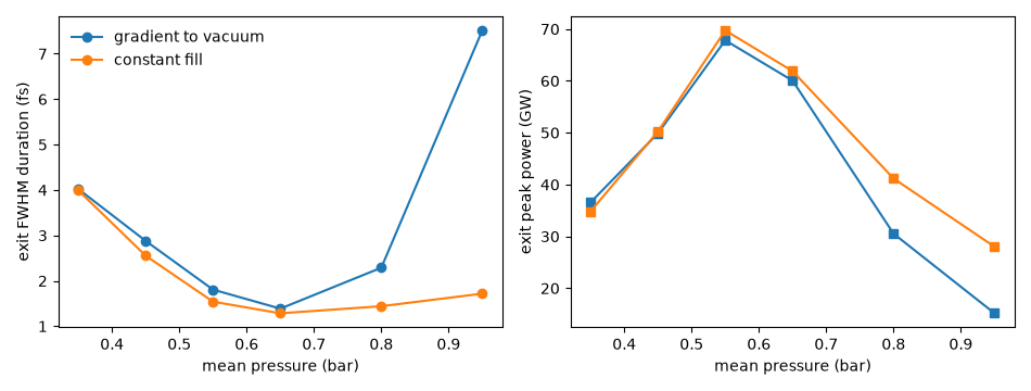
gradient to vacuum mean 0.35 bar:  4.02 fs,   36.6 GW
gradient to vacuum mean 0.45 bar:  2.88 fs,   49.9 GW
gradient to vacuum mean 0.55 bar:  1.81 fs,   67.8 GW
gradient to vacuum mean 0.65 bar:  1.39 fs,   60.0 GW
gradient to vacuum mean 0.80 bar:  2.29 fs,   30.5 GW
gradient to vacuum mean 0.95 bar:  7.51 fs,   15.2 GW
constant fill      mean 0.35 bar:  3.99 fs,   34.8 GW
constant fill      mean 0.45 bar:  2.55 fs,   50.2 GW
constant fill      mean 0.55 bar:  1.54 fs,   69.7 GW
constant fill      mean 0.65 bar:  1.28 fs,   61.9 GW
constant fill      mean 0.80 bar:  1.44 fs,   41.2 GW
constant fill      mean 0.95 bar:  1.72 fs,   28.0 GW

Runtime and reproducibility

Fourteen complete two-metre runs of four coupled modes.

settings = gradient.metadata.backend.settings
print(
    f"{time.perf_counter() - started:.0f} s; backend {gradient.metadata.backend.name}, "
    f"{settings.get('thread_count', 'default')} threads"
)

130 s; backend native, 18 threads

Related reading

Continue with Profiles along the fibre for the model, options and limits, and Assessing numerical accuracy for convergence checks. For a paced propagation lesson, return to Resonant dispersive-wave propagation.