Supercontinuum by soliton self-compression, reaching the vacuum ultraviolet#

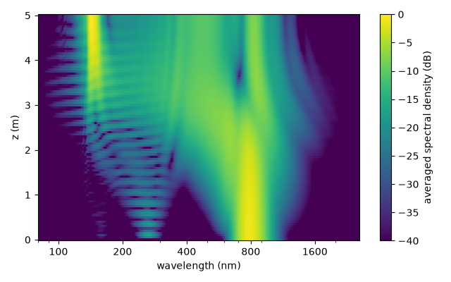
In anomalous dispersion, a sufficiently nonlinear short pulse can self-compress and emit a resonant dispersive wave. Its soliton order depends on power, duration, dispersion and nonlinearity, rather than on energy alone. Here compression produces a broad spectrum, and a seeded ensemble measures how repeatable its amplitude and phase are under the chosen input noise.

This example drives a 5 m capillary of 225 um core radius filled with helium in a pressure gradient falling from 0.2 bar at the entrance to vacuum at the exit, with a 6 fs, 1 mJ pulse at 800 nm. The decreasing gradient accumulates the nonlinear phase near the entrance and strengthens the anomalous dispersion towards the exit, which extends the self-compression; the spectrum reaches below 100 nm.

The ensemble: twenty shots with different realisations of the input shot noise, from which the averaged spectrum, the relative intensity noise (RIN) and the first-order coherence of the exit spectrum are computed.

What to look for. The spectrum explodes where the pulse self-compresses, and a band appears in the vacuum ultraviolet; the coherence stays close to one across the continuum and the RIN small, except at the faintest edges of the spectrum.

What is approximate. Only the fundamental mode is carried; the helium index is optmat’s fit, qualified down to 60 nm, below the band; and the capillary’s loss in the vacuum ultraviolet is the Marcatili approximation. A fitted linear index does not validate the carrier-frequency Kerr coefficient across this bandwidth: the ultraviolet output is also sensitive to the nonlinear-response model. See A frequency-dependent electronic response before interpreting its absolute yield.

The parameter choices follow panel (b) of the supercontinuum figure in the review by Travers et al.; these are regenerated solprop calculations, not the original figure data. The twenty seeded shots sample input optical noise only. They omit technical fluctuations of pulse energy, duration, coupling and gas pressure; convergence of ensemble statistics must be checked for the observable and spectral band of interest.

The ensemble#

Each shot is the same run with a different realisation of the quantum shot noise: one photon per active frequency bin and channel, with a random phase, added to the input spectrum (noise="input"), drawn from the generator seeded by seed.

import time
import warnings

import matplotlib.pyplot as plt
import numpy as np

from solprop.constants import C
from solprop.driver import prop_capillary
from solprop.exceptions import MaterialRangeWarning
from solprop.processing import g12_of, get_spectral_density

SHOTS = 20
"""The size of the ensemble."""

started = time.perf_counter()
runs = []
with warnings.catch_warnings():
    warnings.simplefilter("ignore", MaterialRangeWarning)
    for seed in range(SHOTS):
        runs.append(
            prop_capillary(
                225e-6,
                5.0,
                "He",
                (0.2, 0.0),
                lambda0=800e-9,
                fwhm=6e-15,
                energy=1e-3,
                trange=1e-12,
                wavelength_limits=(80e-9, 4e-6),
                noise="input",
                seed=seed,
                n_save=101,
                progress="none",
            )
        )

The averaged spectrum along the fibre#

The spectral energy density averaged over the ensemble, in decibels below its peak.

z = np.asarray(runs[0]["z"])
spectra = []
for run in runs:
    wavelength, density = get_spectral_density(run, "wavelength")
    spectra.append(density)
spectra = np.asarray(spectra)  # (shots, planes, wavelengths)
mean = spectra.mean(axis=0)
shown = (wavelength > 80e-9) & (wavelength < 2.6e-6)
ticks = [100, 200, 400, 800, 1600]  # nm, labelled in full on the log axis

fig, ax = plt.subplots(figsize=(6.4, 4.0))
image = ax.pcolormesh(
    wavelength[shown] * 1e9,
    z,
    10 * np.log10(np.maximum(mean[:, shown] / mean.max(), 1e-12)),
    vmin=-40,
    vmax=0,
    shading="auto",
)
ax.set_xscale("log")
ax.set_xticks(ticks, labels=[str(tick) for tick in ticks])
ax.tick_params(axis="x", which="minor", labelbottom=False)
ax.set_xlabel("wavelength (nm)")
ax.set_ylabel("z (m)")
fig.colorbar(image, ax=ax, label="averaged spectral density (dB)")
fig.tight_layout()

Noise and coherence at the exit#

From top to bottom: the exit spectra of every shot (grey) and their mean (black); the relative intensity noise, the standard deviation of the spectral density over its mean, shot to shot; and the first-order coherence \(|g_{12}^{(1)}(\lambda)|\) of the ensemble’s complex spectra (0 for independent fields, 1 for identical ones).

exit_mean = spectra[:, -1].mean(axis=0)
rin = spectra[:, -1].std(axis=0) / exit_mean
omega, coherence = g12_of(runs, plane=-1)
coherent_wavelength = 2 * np.pi * C / omega
significant = exit_mean > 1e-4 * exit_mean[shown].max()

fig, (top, middle, bottom) = plt.subplots(3, 1, figsize=(6.4, 7.5), sharex=True)
for shot in spectra[:, -1]:
    top.semilogy(wavelength[shown] * 1e9, shot[shown], color="0.75", linewidth=0.5)
top.semilogy(wavelength[shown] * 1e9, exit_mean[shown], color="k", linewidth=1.0)
top.set_ylim(1e-6 * exit_mean[shown].max(), 3 * exit_mean[shown].max())
top.set_ylabel("spectral density (J/m)")
keep = shown & significant
middle.semilogy(wavelength[keep] * 1e9, rin[keep], color="tab:red", linewidth=1.0)
middle.set_ylabel("RIN")
in_window = (coherent_wavelength > 80e-9) & (coherent_wavelength < 2.6e-6)
bottom.plot(
    coherent_wavelength[in_window] * 1e9, coherence[in_window], color="tab:blue"
)
bottom.set_ylim(0, 1.05)
bottom.set_ylabel("coherence $|g_{12}|$")
bottom.set_xscale("log")
bottom.set_xticks(ticks, labels=[str(tick) for tick in ticks])
bottom.tick_params(axis="x", which="minor", labelbottom=False)
bottom.set_xlabel("wavelength (nm)")
fig.tight_layout()

weights = exit_mean[shown] / exit_mean[shown].sum()
mean_rin = float(np.sum(weights * np.nan_to_num(rin[shown])))
on_grid = np.interp(wavelength[shown], coherent_wavelength[::-1], coherence[::-1])
mean_coherence = float(np.nansum(weights * on_grid))
print(
    f"{len(runs)} shots; spectrally weighted RIN {mean_rin:.3e}, "
    f"spectrally weighted coherence {mean_coherence:.12f}"
)

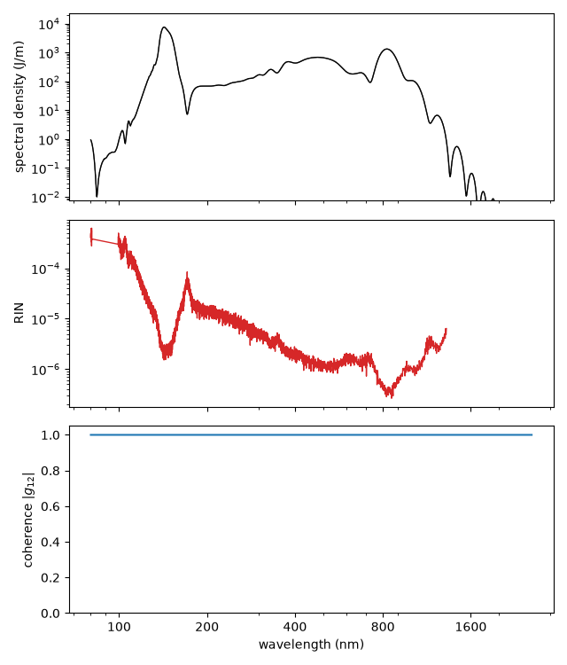
20 shots; spectrally weighted RIN 3.758e-06, spectrally weighted coherence 0.999999999934

Runtime and reproducibility#

print(
    f"{time.perf_counter() - started:.0f} s for {len(runs)} shots; "
    f"backend {runs[0].metadata.backend.name}"
)

167 s for 20 shots; backend native