Self-phase modulation and post-compression

A common use of a gas-filled hollow capillary is post-compression: a femtosecond pulse is spectrally broadened by self-phase modulation (SPM) in the gas, and the broadened, chirped pulse is then compressed with a dispersive delay line – chirped mirrors, prisms or gratings – to a duration far below the input’s.

The Kerr effect makes the refractive index depend on the instantaneous intensity, \(n = n_0 + n_2 I(t)\), so the pulse writes a time-dependent phase \(\phi(t) = +k_0 n_2 I(t) L\) onto itself in the optics convention. The frequency shift is \(\delta\omega=-\partial_t\phi\): the leading edge is shifted to the red and the trailing edge to the blue, so the spectrum broadens in proportion to the peak nonlinear phase. In argon at a few bar the dispersion of the gas-filled capillary is normal at 800 nm, so the pulse stretches slightly as it broadens and the chirp stays nearly linear across its centre, which is what makes the output compressible. The intensity dependence of the group velocity, self-steepening, tilts the pulse so that its trailing edge sharpens and the blue side of the spectrum extends further than the red.

The parameters are those of a standard compressor: a 30 fs, 250 uJ pulse at 800 nm in a 0.75 m capillary of 125 um core radius filled with argon at 5 bar. Photoionisation is switched off to isolate the Kerr effect.

What to look for. The spectrum broadens symmetrically at first, then develops the characteristic SPM fringes and a blue shoulder from self-steepening; in time the pulse broadens and steepens at its trailing edge. At this energy the spectrum spans more than an octave, and its transform-limited pulse – what an ideal compressor would give – is under two femtoseconds, more than an order of magnitude shorter than the input; a compressor that corrects only the second- and third-order spectral phase already reaches about two thirds of that limit’s peak power.

What is approximate. Only the fundamental HE_11 mode is carried and the plasma is off, so this is the pure Kerr limit; at higher energies ionisation and coupling to higher-order modes become important. The gas index is scaled linearly with density, which at 5 bar of argon departs from optmat’s finite-density law by about \(10^{-3}\) of \(n - 1\) in the deep ultraviolet; the run records the error in its material manifest, below the 1 % at which it would warn (DiluteScalingWarning).

This is panel (a) of the survey of nonlinear processes in hollow-core fibres in J. C. Travers, T. Grigorova, C. Brahms and F. Belli, “Nonlinear optics in gas-filled hollow-core optical fibers” (review).

For the response and phase conventions see Nonlinear responses. The offline-compression guide explains what phase-only optimisation can recover from the broadened spectrum.

The run

import time

import matplotlib.pyplot as plt

from solprop.driver import prop_capillary
from solprop.plotting import prop_2d, spec_1d, time_1d
from solprop.processing import compress_taylor

started = time.perf_counter()
run = prop_capillary(
    125e-6,
    0.75,
    "Ar",
    5.0,
    lambda0=800e-9,
    fwhm=30e-15,
    energy=250e-6,
    plasma=False,
    trange=700e-15,
    wavelength_limits=(200e-9, 4e-6),
    n_save=301,
    progress="none",
)

Spectral and temporal evolution

figures = prop_2d(
    run,
    "wavelength",
    wavelength_range=(200e-9, 3e-6),
    trange=(-150e-15, 250e-15),
    db_min=-40,
)
figures[-1].set_size_inches(9.5, 3.6)
figures[-1].tight_layout()

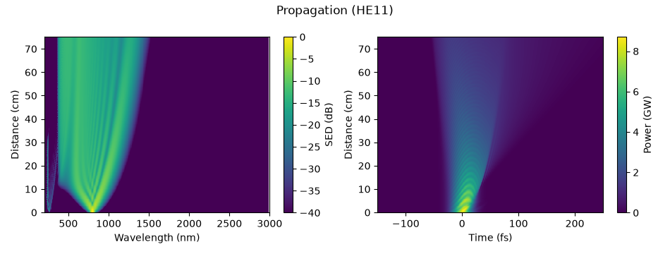
The output, and what a compressor makes of it

On the left, the output pulse as it leaves the fibre, its transform limit, and the pulse after the best Taylor-phase compression (group-delay dispersion and third-order dispersion) of the output spectrum. On the right, the input and output spectra.

compressed = compress_taylor(run, order=3)
fig, (left, right) = plt.subplots(1, 2, figsize=(10.0, 3.6))
time_1d(run, trange=(-150e-15, 250e-15), ax=left, widths=False)
time_1d(run, trange=(-150e-15, 250e-15), ax=left, transform_limit=True, widths=False)
time_1d(
    run, trange=(-150e-15, 250e-15), ax=left, transfer=compressed.transfer, widths=False
)
left.legend(["output", "transform limit", "Taylor-compressed"], frameon=False)
spec_1d(run, z=[0.0, 0.75], ax=right, wavelength_range=(300e-9, 2e-6))
fig.tight_layout()

before, after = compressed.fwhm_before * 1e15, compressed.fwhm_after * 1e15
print(
    f"input 30 fs; output {before:.1f} fs; transform limit "
    f"{compressed.fwhm_limit * 1e15:.1f} fs; compressed {after:.1f} fs, "
    f"{compressed.quality:.0%} of the transform-limited peak power"
)
print(compressed)

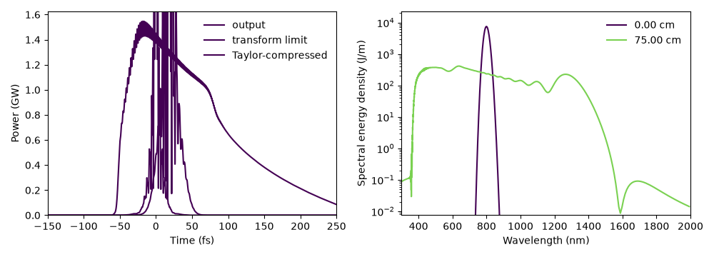
input 30 fs; output 132.4 fs; transform limit 1.6 fs; compressed 2.0 fs, 67% of the transform-limited peak power
Compression by taylor
  found:      GDD -61.25 fs^2, TOD -18.51 fs^3
  duration:   132.4 fs before, 1.951 fs after, 1.554 fs at the transform limit
  peak power: 1.547 GW before, 85.52 GW after, 127.4 GW at the limit
  quality:    0.6715 of the transform-limited peak power
  search:     converged: Optimization terminated successfully. (2645 evaluations)

Runtime and reproducibility

print(f"{time.perf_counter() - started:.0f} s; backend {run.metadata.backend.name}")

5 s; backend native