Note
Go to the end to download the full example code.
Gas flow in a hollow fibre: tapers, choked ends and the flow regime#
A gradient fill is a steady flow between two gas cells. For laminar flow of an
isothermal ideal gas, the mass flow a^4 p dp/dz is the same everywhere, so p^2
is linear in the hydraulic resistance int a^-4 dz (Pennetta et al., APL Photonics
4, 056105 (2019), eq. 6): a narrow section carries most of the pressure drop. An end
pumped to vacuum cannot pass more gas than leaves it at the speed of sound, so it
chokes at a pressure well above zero. And the laminar law has limits: above a
Reynolds number of about 2000 the flow is no longer laminar, and Gebhardt et al.
(Opt. Express 29, 6957 (2021)) measured output-beam instabilities from 2040.
This tutorial builds fills with solprop.gasflow.steady_fill() and reads their
FlowReport. Nothing is propagated; see
Profiles along the fibre for the derivation and for how the choked pressure
compares
with an integration of the compressible flow. The choked pressure uses the adiabatic
sound speed at the fill temperature, which puts it between the values for an
isothermal and an adiabatic wall: for the cases checked there, an integration with an
isothermal wall gives 16-25 % more and one with an adiabatic wall 10-16 % less.
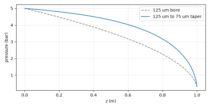
A tapered fill against a uniform one. The taper narrows from 125 um to 75 um along a metre of argon between 5 bar and a pumped end. Both ends choke, at similar pressures: the taper’s narrow exit would raise its choked pressure (less area for the sonic throughput), and its larger resistance lowers it (less throughput to pass).
import matplotlib.pyplot as plt
import numpy as np

from solprop.gasflow import choked_pressure, flow_report, steady_fill
from solprop.profiles import Linear, PiecewiseLinear

length = 1.0
taper = Linear(125e-6, 75e-6, length)
uniform = steady_fill("Ar", [0.0, length], [5.0, 0.0], radius=125e-6)
tapered = steady_fill("Ar", [0.0, length], [5.0, 0.0], radius=taper)

z = np.linspace(0.0, length, 401)
fig, axis = plt.subplots(figsize=(7.0, 3.6))
axis.plot(z, uniform(z), color="0.5", linestyle="--", label="125 um bore")
axis.plot(z, tapered(z), color="C0", label="125 um to 75 um taper")
axis.set_xlabel("z (m)")
axis.set_ylabel("pressure (bar)")
axis.legend()
axis.grid(alpha=0.3)
fig.tight_layout()

for name, fill in (("uniform", uniform), ("tapered", tapered)):
    print(f"{name:8s} exit pressure {fill.pressures[-1] * 1e3:6.1f} mbar")
/home/docs/checkouts/solprop/checkouts/24/docs/tutorials/capillaries/plot_03_gas_flow.py:42: GasFlowWarning: the steady-flow fill has a peak Reynolds number of 2005 at z = 0 m, above 2000: the laminar fill is not valid there, and output-beam instabilities have been measured in differentially pumped capillaries from Re = 2040, worst near 2400 (Gebhardt et al., Opt. Express 29, 6957 (2021)). Lower the pressure difference or widen the bore
  uniform = steady_fill("Ar", [0.0, length], [5.0, 0.0], radius=125e-6)
uniform  exit pressure  341.9 mbar
tapered  exit pressure  314.2 mbar
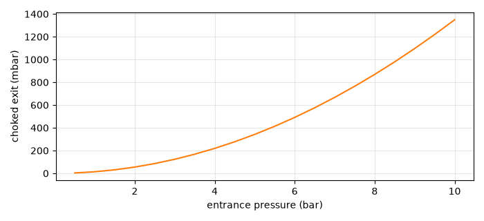
The choked end. The exit pressure solves k (p_h^2 - p_e^2) = p_e with
k = 1 / (16 eta c a_e^2 R); for the uniform bore it grows as the square of the
entrance pressure while the exit stays much lower than the entrance.
entrance = np.linspace(0.5, 10.0, 20)
exit_pressure = [choked_pressure("Ar", 125e-6, length, p) for p in entrance]
fig, axis = plt.subplots(figsize=(7.0, 3.2))
axis.plot(entrance, np.array(exit_pressure) * 1e3, color="C1")
axis.set_xlabel("entrance pressure (bar)")
axis.set_ylabel("choked exit (mbar)")
axis.grid(alpha=0.3)
fig.tight_layout()
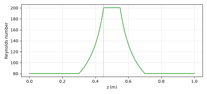
The Reynolds number along a waist. The mass flow is constant along a stage and
Re = 2 mdot / (pi a eta), so the narrowest point has the largest Reynolds number.
The report gives each stage’s throughput, mass flow, peak Reynolds number and
Knudsen numbers, and whether each outer end is choked.
waist = PiecewiseLinear.from_stages(
    [0.0, 0.3, 0.45, 0.55, 0.7, 1.0], [150e-6, 150e-6, 60e-6, 60e-6, 150e-6, 150e-6]
)
fill = steady_fill("Ar", [0.0, length], [2.0, 0.0], radius=waist)
report = flow_report(fill, "Ar", radius=waist)
print(report)

stage = report.stages[0]
reynolds = 2.0 * stage.mass_flow / (np.pi * waist(z) * report.viscosity)
fig, axis = plt.subplots(figsize=(7.0, 3.2))
axis.plot(z, reynolds, color="C2")
axis.axvline(stage.peak_reynolds_position, color="0.6", linestyle=":")
axis.set_xlabel("z (m)")
axis.set_ylabel("Reynolds number")
axis.grid(alpha=0.3)
fig.tight_layout()
plt.show()
FlowReport: steady laminar flow
  viscosity:   22.29 uPa s
  sound speed: 318.9 m/s
  0 m to 1 m:  0.2569 mbar l/s, 0.01417 slpm, peak Re 200.4 at 450 mm, peak Kn 0.0202
  end:         choked (choked pressure 0.0114 bar)