Note
Go to the end to download the full example code.
A tapered capillary: compression, a dispersive wave and mode conversion#
A capillary whose bore narrows along its length is a second handle on soliton dynamics beside the fill. Narrowing the core raises the intensity for the same energy, which accelerates self-compression, and strengthens the waveguide’s anomalous dispersion, which moves the zero-dispersion wavelength – and with it the resonant dispersive wave – towards shorter wavelengths.
A taper also does something a straight bore cannot: it converts between modes.
The field is written on the modes of the local bore, and those modes change shape
as the bore narrows, so propagating in them costs a term, the connection
C_mn = (a'/a) 2 s_m s_n u_m u_n / (u_m^2 - u_n^2)
(Mode conversion in a capillary taper). prop_capillary carries it by default on
every
multimode taper, with or without wall=CoherentWall(); the wall adds its own
coherent loss on top. taper_coupling=False is the adiabatic approximation,
each mode following its local shape without linear taper conversion, which
this example runs beside the coupled taper for comparison.
The fibre here is a metre of helium-filled capillary: 50 cm of 100 um core radius, a
linear taper to 60 um over the next 20 cm, and 30 cm at 60 um. The pump is a 10 fs,
150 uJ pulse at 800 nm. All runs carry four HE_1m modes. First, at a nanojoule,
where nonlinear transfer is negligible for this comparison, the taper three times:
with the
coherent wall, without it
(the connection alone) and adiabatically; this isolates the linear conversion and
separates the connection’s share from the wall’s. Then at full energy, three times:
the taper with the coherent wall, the same taper adiabatically, with each mode’s own
Marcatili loss and no wall, and the straight 100 um bore with the wall.
What to look for. In the linear runs the coherent wall alone holds a few parts
in a million of the launch in HE_12 to HE_14 along the straight bore – the
coherent exchange a lossy boundary makes between modes – and HE_12 then jumps
by a factor of twenty or more at the start of the transition, where the connection
switches on; the taper without the wall makes the same jump there, having held
nothing in the straight bore, so the jump is the connection’s, and the adiabatic run
leaves every higher mode below 1e-13. At full
energy the pulse compresses and emits its dispersive wave in the narrow section,
earlier than in the straight bore and further into the ultraviolet; there the Kerr
overlap between the modes moves far more energy into the higher modes than the taper
does, from the first centimetre, so the connection shows only in the weakest
channel.
What is approximate. The taper connection is derived for the Dirichlet
J_0 basis the capillary modes are built on, and it is exact for that basis;
the coherent wall is the condensed paraxial Robin condition, and its validity ratios
are printed from the run’s record (the run warns when the quasi-static one comes
within a factor ten of its limit, as it does in the 60 um section at the longest
wavelengths). The gas index is optmat’s helium fit, qualified over the whole band
(from 60 nm).
The set-up#
The taper is a PiecewiseLinear profile of the core
radius. Its corners are where the linear operator’s intervals begin and end, and
the adaptive stepper lands on each of them.
import time
import warnings

import matplotlib.pyplot as plt
import numpy as np

from solprop.driver import prop_capillary
from solprop.exceptions import (
    AdiabaticTaperWarning,
    GrazingIncidenceWarning,
    SolpropWarning,
)
from solprop.modes import CoherentWall
from solprop.plotting import prop_2d
from solprop.processing import (
    bandpass,
    fwhm_t,
    get_spectral_density,
    grid_of,
)
from solprop.processing import energy as energy_of
from solprop.processing import peak_power as peak_power_of
from solprop.profiles import PiecewiseLinear

LENGTH = 1.0
"""Capillary length, m."""

CORNERS = (0.0, 0.5, 0.7, LENGTH)
"""Where the straight, tapering and straight sections meet, m."""

TAPER = PiecewiseLinear.from_stages(CORNERS, [100e-6, 100e-6, 60e-6, 60e-6])
"""Core radius along z, m."""

PRESSURE = 1.5
"""Helium pressure, bar."""

PUMP = {"lambda0": 800e-9, "fwhm": 10e-15, "energy": 150e-6}
"""The pump: wavelength (m), duration (s) and energy (J)."""

UV = (100e-9, 300e-9)
"""The band the dispersive wave is counted in, m."""

started = time.perf_counter()


def propagate(radius, wall, backend="auto", energy=PUMP["energy"], taper_coupling=True):
    """Propagate the pump along `radius`, with or without the wall and the coupling."""
    with warnings.catch_warnings():
        # The wall's quasi-static ratio approaches its limit at the longest
        # wavelengths of the narrow section: the approximation named above, which
        # each run would repeat. An AdiabaticTaperWarning would name the comparison
        # this example draws on purpose, so it is silenced too. The coherent
        # wall's generator is resolved along z to a Chebyshev tail at the round-off
        # floor of its samples, which it reports as a SolpropWarning.
        for category in (
            GrazingIncidenceWarning,
            AdiabaticTaperWarning,
            SolpropWarning,
        ):
            warnings.simplefilter("ignore", category)
        return prop_capillary(
            radius,
            LENGTH,
            "He",
            PRESSURE,
            wavelength_limits=(90e-9, 3e-6),
            trange=250e-15,
            modes=4,
            wall=wall,
            taper_coupling=taper_coupling,
            dz_max=2e-3,
            n_save=200,
            progress="none",
            backend=backend,
            lambda0=PUMP["lambda0"],
            fwhm=PUMP["fwhm"],
            energy=energy,
        )


def shares(run):
    """Return the positions and each mode's energy over the launched energy."""
    per_mode = np.asarray(energy_of(run))
    return np.asarray(run["z"]), per_mode / per_mode[0].sum()
The linear conversion#
One nanojoule, so that the Kerr effect is ten orders of magnitude below everything else. With the coupling declined, the adiabatic taper’s multimode set on a radius profile with corners is carried by the linear operator’s general z table, which every CPU backend runs (the native backend evaluates it in its own kernels at each step’s positions), so the default backend runs it too. The coupled runs, with or without the wall, carry the taper in the coupled flow instead.
linear = {
    "coherent wall": propagate(TAPER, CoherentWall(), energy=1e-9),
    "no wall (coupled)": propagate(TAPER, None, energy=1e-9),
    "no wall (adiabatic)": propagate(TAPER, None, energy=1e-9, taper_coupling=False),
}
fig, ax = plt.subplots(figsize=(6.4, 4.0))
for (name, run), style in zip(linear.items(), ("-", "--", ":"), strict=True):
    z, fraction = shares(run)
    for mode in range(1, 4):
        ax.semilogy(
            z,
            np.maximum(fraction[:, mode], 1e-30),
            style,
            color=f"C{mode}",
            label=f"HE_1{mode + 1}, {name}",
        )
for corner in CORNERS[1:3]:
    ax.axvline(corner, color="0.5", linewidth=0.8, linestyle="--")
ax.set_ylim(1e-14, 1e-1)
ax.set_xlabel("z (m)")
ax.set_ylabel("fraction of the launched energy")
ax.set_title("1 nJ: the conversion is the taper's")
ax.legend(frameon=False, fontsize="x-small", ncol=3)
fig.tight_layout()

# **Check the weak channel near the taper corner.** A spurious spike in a
# nearly empty mode can be hidden by good conservation of total energy. The coupled
# flow applies its explicit residual only on the requested band; the spectral collar
# around it is carried by each section's frozen block alone. Were the residual
# applied in the collar too, the plane at z = 0.6985 m, just before the transition
# ends, would show HE14 a thousand times above its neighbours, a numerical artefact
# rather than a conversion. Compare
# that plane's HE14 share with its neighbours'. Smoothness is a useful diagnostic,
# but does not replace step, band and mode-count refinement; see
# :doc:`/guide/numerics/accuracy`.

for name, run in linear.items():
    z, fraction = shares(run)
    near = int(np.argmin(np.abs(z - 0.6985)))
    around = ", ".join(
        f"z = {z[index]:.4f} m {fraction[index, 3]:.2e}"
        for index in (near - 5, near, near + 5)
    )
    print(f"{name:20s} HE_14 near the corner: {around}")

for name, run in linear.items():
    z, fraction = shares(run)
    before = int(np.argmin(np.abs(z - CORNERS[1])))
    after = int(np.argmin(np.abs(z - (CORNERS[2] + 0.01))))
    for label, index in (("z = 0.5 m", before), ("z = 0.71 m", after)):
        text = ", ".join(
            f"HE_1{m + 2} {share:.2e}" for m, share in enumerate(fraction[index, 1:])
        )
        print(f"{name:20s} {label:9s} {text}")
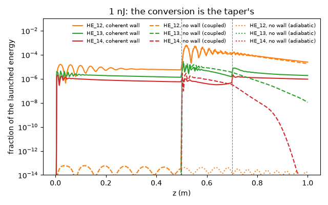
coherent wall        HE_14 near the corner: z = 0.6734 m 3.60e-07, z = 0.6985 m 4.59e-07, z = 0.7236 m 1.52e-06
no wall (coupled)    HE_14 near the corner: z = 0.6734 m 4.40e-07, z = 0.6985 m 3.35e-07, z = 0.7236 m 1.58e-07
no wall (adiabatic)  HE_14 near the corner: z = 0.6734 m 9.60e-20, z = 0.6985 m 8.80e-20, z = 0.7236 m 7.31e-20
coherent wall        z = 0.5 m HE_12 2.67e-05, HE_13 5.56e-06, HE_14 1.13e-06
coherent wall        z = 0.71 m HE_12 1.71e-04, HE_13 7.74e-06, HE_14 1.49e-06
no wall (coupled)    z = 0.5 m HE_12 2.50e-05, HE_13 7.25e-06, HE_14 2.77e-06
no wall (coupled)    z = 0.71 m HE_12 1.28e-04, HE_13 3.01e-06, HE_14 2.54e-07
no wall (adiabatic)  z = 0.5 m HE_12 4.05e-14, HE_13 2.75e-15, HE_14 1.40e-19
no wall (adiabatic)  z = 0.71 m HE_12 1.54e-14, HE_13 1.71e-15, HE_14 7.48e-20
The nonlinear runs#
The same fibre at 150 uJ, with and without the wall, and the straight bore.
What the record says about the flow: how many frozen sections the run was cut into, the Chebyshev degree along z the wall’s generator was resolved at, whether the connection was carried (it is, because the radius varies), the advisory step, and the worst of the three validity ratios over the whole run.
model          mean impedance coherent wall
n_sections     4
n_deg          17
connection     True
advisory_step  0.000167777
quasi_static   0.0952
The walled taper’s propagation map, summed over the modes. The spectrum broadens slowly along the straight section and explodes at the end of the taper, where the pulse compresses and the dispersive wave appears near 130 nm.
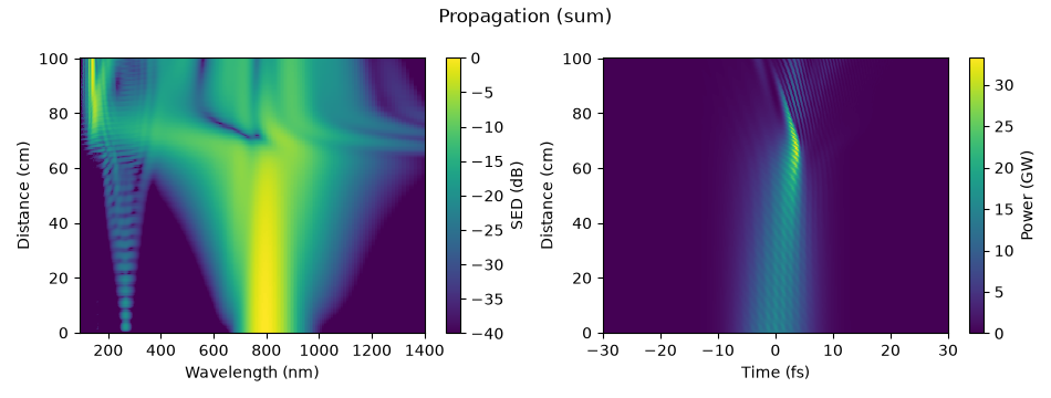
Compression along the fibre#
The peak of the total power: the taper compresses the pulse earlier than the straight bore does, because it squeezes the same energy into a smaller area.
fig, ax = plt.subplots(figsize=(6.4, 3.6))
for name, run in runs.items():
    ax.plot(np.asarray(run["z"]), peak_power_of(run, modes="sum") * 1e-9, label=name)
for corner in CORNERS[1:3]:
    ax.axvline(corner, color="0.5", linewidth=0.8, linestyle="--")
ax.set_xlabel("z (m)")
ax.set_ylabel("peak power (GW)")
ax.legend(frameon=False, fontsize="small")
fig.tight_layout()

for name, run in runs.items():
    power = peak_power_of(run, modes="sum")
    best = int(np.argmax(power))
    print(
        f"{name:31s} peak {power[best] * 1e-9:6.1f} GW at z = "
        f"{np.asarray(run['z'])[best]:.3f} m, "
        f"{fwhm_t(run, plane=best, modes='sum') * 1e15:.2f} fs there"
    )
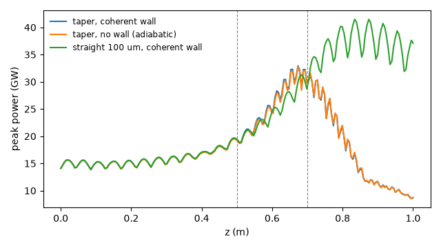
taper, coherent wall            peak   32.9 GW at z = 0.673 m, 1.79 fs there
taper, no wall (adiabatic)      peak   32.7 GW at z = 0.673 m, 1.80 fs there
straight 100 um, coherent wall  peak   41.5 GW at z = 0.834 m, 1.62 fs there
Mode conversion at full energy#
The energy in each mode along the fibre, as a fraction of the launched energy.
The Kerr overlap between the modes fills HE_12 and HE_13 to 1e-3 within
the first centimetre, in both runs, and the compression in the narrow section
moves more; against that, the taper’s own conversion – the linear figure above –
is visible only in HE_14, which the wall and the connection hold an order of
magnitude above the adiabatic run before the taper and through it.
fig, ax = plt.subplots(figsize=(6.4, 4.0))
for name, style in (("taper, coherent wall", "-"), ("taper, no wall (adiabatic)", ":")):
    run = runs[name]
    z = np.asarray(run["z"])
    per_mode = np.asarray(energy_of(run))
    launched = per_mode[0].sum()
    for mode in range(1, 4):
        ax.semilogy(
            z,
            np.maximum(per_mode[:, mode] / launched, 1e-20),
            style,
            color=f"C{mode}",
            label=f"HE_1{mode + 1}, {name.split(', ')[1]}",
        )
for corner in CORNERS[1:3]:
    ax.axvline(corner, color="0.5", linewidth=0.8, linestyle="--")
ax.set_ylim(1e-12, 1e-1)
ax.set_xlabel("z (m)")
ax.set_ylabel("fraction of the launched energy")
ax.legend(frameon=False, fontsize="small", ncol=2)
fig.tight_layout()
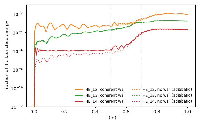
The same numbers at two places: just after the transition (z = 0.71 m), before the pulse has compressed, where the difference is the connection alone, and at the exit.
for name in ("taper, coherent wall", "taper, no wall (adiabatic)"):
    run = runs[name]
    per_mode = np.asarray(energy_of(run))
    z = np.asarray(run["z"])
    end_of_taper = int(np.argmin(np.abs(z - (CORNERS[2] + 0.01))))
    for label, index in (("z = 0.71 m", end_of_taper), ("exit", -1)):
        shares = per_mode[index] / per_mode[0].sum()
        text = ", ".join(f"HE_1{m + 1} {share:.2e}" for m, share in enumerate(shares))
        print(f"{name:27s} {label:9s} {text}")
taper, coherent wall        z = 0.71 m HE_11 5.86e-01, HE_12 2.66e-03, HE_13 1.29e-03, HE_14 1.06e-04
taper, coherent wall        exit      HE_11 2.68e-01, HE_12 8.63e-03, HE_13 1.76e-03, HE_14 2.07e-04
taper, no wall (adiabatic)  z = 0.71 m HE_11 5.89e-01, HE_12 2.30e-03, HE_13 1.22e-03, HE_14 9.58e-05
taper, no wall (adiabatic)  exit      HE_11 2.67e-01, HE_12 8.68e-03, HE_13 1.70e-03, HE_14 1.94e-04
The dispersive wave#
The exit spectra, summed over the modes. The narrower core pushes the dispersive wave further into the ultraviolet than the straight bore does, and the energy in the ultraviolet band is printed below.
fig, ax = plt.subplots(figsize=(6.4, 3.6))
for name, run in runs.items():
    wavelength, density = get_spectral_density(run, "wavelength", plane=-1, modes="sum")
    order = np.argsort(wavelength)
    ax.semilogy(wavelength[order] * 1e9, density[order], label=name, linewidth=1.0)
ax.set_xlim(100.0, 1200.0)
ax.set_ylim(1e-4 * np.max(density), 3.0 * np.max(density))
ax.set_xlabel("wavelength (nm)")
ax.set_ylabel("spectral energy density (J/m)")
ax.legend(frameon=False, fontsize="small")
fig.tight_layout()

for name, run in runs.items():
    launched = float(np.sum(energy_of(run, plane=0)))
    uv = float(np.sum(energy_of(run, plane=-1, bandpass=bandpass(grid_of(run), UV))))
    left = float(np.sum(energy_of(run, plane=-1)))
    print(
        f"{name:31s} transmitted {left / launched:.3f}; "
        f"100-300 nm {uv * 1e6:.2f} uJ ({uv / launched:.2%})"
    )
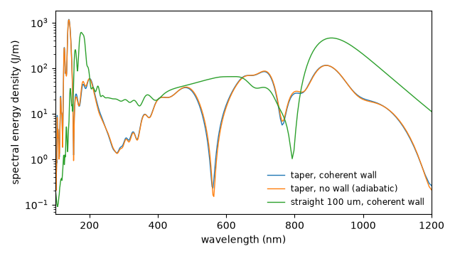
taper, coherent wall            transmitted 0.279; 100-300 nm 14.01 uJ (9.34%)
taper, no wall (adiabatic)      transmitted 0.278; 100-300 nm 13.72 uJ (9.14%)
straight 100 um, coherent wall  transmitted 0.705; 100-300 nm 16.79 uJ (11.19%)
Runtime and reproducibility#
Six complete one-metre runs of four coupled modes: three linear, three nonlinear.
55 s; backend native, 18 threads