Far-field spectra through apertures

A spectrometer behind a nonlinear sample rarely sees the whole beam: the light crosses a distance, or a lens, and part of it enters through a hole. This tutorial records what such detectors measure, at every saved plane of a free-space run, without storing the field there (Plane statistics, Far-field apertures and angular regions):

• aperture_spectrum, the spectrum through each hole of an ApertureSet in a mask plane;

• region_spectrum, the spectrum in boxes of transverse wavevector, here the four quadrants;

• beam_spectrum, the whole beam’s spectrum;

• absorbed_power, what the absorbers remove per unit length, sampled every step.

Two equal pulses cross at a small angle in a thin Kerr sample, as in A four-wave-mixing delay scan through one backend, and each diffracts from the grating they write into a new direction. Holes in a mask plane catch the two beams, one of the four-wave-mixing signals and a dark spot where no light should arrive. The tutorial shows the paraxial map that places each frequency in the mask plane, the chromatic weight an aperture applies, the two edge weightings against a closed form, and checks the run’s statistic against a computation from a kept field. Every spectrum is the axial Poynting flux inside the sample, in its medium (Energy and flux in a medium).

The sample and the grid

The pulses are 50 fs long at 800 nm with a 40 μm waist and a peak field of \(7.51\times10^8\) V/m each, about 0.145 μJ each in the sample (printed below); the sample is 1 mm of a dispersionless medium of index 1.45 with an illustrative nonlinear index of \(3\times10^{-20}\) m²/W. Inside it the beams travel at \(\pm10\) mrad, transverse wavenumbers \(\pm K_0\); the signal \(2\mathbf k_1-\mathbf k_2\) leaves at \(3K_0\).

Two grid choices matter for far-field statistics. The spacing keeps the cubic products from folding back (the one-half rule of Cartesian free-space propagation asks for \(k_{x,\max}>7K_0\)). The box decides how finely the far field is sampled: a stored column is one direction, and neighbouring columns land \(s(\omega)\Delta\kappa\) apart in the mask plane, \(s=z_mc/\omega\). A box of 0.8 mm, twenty waists, puts six lattice points across the far-field radius.

import time

import matplotlib.pyplot as plt
import numpy as np
from matplotlib.patches import Circle
from scipy import integrate

from solprop.boundaries import TransverseCollar, absorber, custom_absorber
from solprop.constants import C
from solprop.driver import SimulationSettings, prop_free
from solprop.grid import EnvelopeGrid, FreeGrid
from solprop.nonlinear.responses import KerrResponse
from solprop.output.schema import SavedPlane
from solprop.physdata.nonlinear_data import chi3_from_n2
from solprop.pulses import GaussianPulse
from solprop.spatial import (
    SpatialFlux,
    SpatialMedium,
    aperture_profile,
    quadrature_half_width,
    spatial_energy,
)
from solprop.stats import ApertureSet, StatsSpec, collect
from solprop.stepper import FixedSchedule, PIController

started = time.perf_counter()
LENGTH = 1e-3
WAVELENGTH = 800e-9
INDEX = 1.45
N2 = 3e-20
WAIST = 40e-6
FIELD = 7.5051e8  # V/m, the peak of each beam's analytic field
FWHM = 50e-15
ANGLE = 0.010
K0 = 2 * np.pi * INDEX / WAVELENGTH * np.sin(ANGLE)
grid = EnvelopeGrid.from_limits(LENGTH, WAVELENGTH, (740e-9, 870e-9), 300e-15)
space = FreeGrid(0.4e-3, 224, 0.4e-3, 64, window_factor=0.0)
k_max = float(np.max(np.abs(space.k_x)))
print(f"K0/k_max = {K0 / k_max:.2f}; grid {space.n_x} x {space.n_y} x {grid.n_omega}")

K0/k_max = 0.13; grid 224 x 64 x 128

The launch

Each beam is the transverse DFT of its field in the internal FFT convention, whose tilt carries a minus sign: beam 1 travels towards positive x (Two crossing beams in Cartesian free space). The tilt is achromatic, a fixed angle at every frequency. Each beam is stated by its physical field, a Gaussian times a temporal envelope of unit peak scaled to FIELD, and its energy is measured in the sample’s medium.

def beam(direction):
    """One tilted Gaussian beam of peak field FIELD on the grid."""
    x, y = np.meshgrid(space.x, space.y)
    pulse = GaussianPulse(wavelength=WAVELENGTH, fwhm=FWHM, peak_power=1.0)
    profile = np.exp(-(x**2 + y**2) / WAIST**2)
    tilt = np.exp(
        -1j * direction * x[..., None] * grid.omega * INDEX * np.sin(ANGLE) / C
    )
    physical = FIELD * profile[..., None] * tilt * pulse.build(grid)[0, 0]
    return np.fft.fft2(physical, axes=(0, 1)).reshape(-1, 1, grid.n_omega)


sample = SpatialMedium(INDEX)
entrance = SpatialFlux.resolve(grid, space, sample)
exit_plane = SpatialFlux.resolve(grid, space, sample, z=LENGTH)
launch = beam(+1) + beam(-1)
print(f"each beam carries {spatial_energy(beam(+1), entrance) * 1e6:.4f} μJ")

each beam carries 0.1450 μJ

The detectors

The mask plane is 0.25 m behind the exit face (or the back focal plane of a lens of that focal length). A beam of transverse wavevector \(\boldsymbol\kappa\) leaves the face at \(\sin\theta=c|\boldsymbol\kappa|/\omega\) whatever the medium, so the beams land at \(\pm X\) with \(X=z_mcK_0/\omega_0\), the signal at \(3X\), all at every frequency. Four holes of the same raised-cosine profile share the set: three on those images and a “dark” hole off the plane of incidence, where no product of the two beams’ directions can go. They use quadrature weighting, so each smooth hole stands in for a hard hole of the same diameter (the raised cosine is the recommended profile for it).

The four quadrants tile the plane of transverse wavevector. Every position and wavevector given is physical, positive for light travelling towards positive x.

DISTANCE = 0.25
X = DISTANCE * C * K0 / grid.omega0
centres = [[X, 0.0], [-X, 0.0], [3 * X, 0.0], [0.0, 1.6 * X]]
diameters = [2.4e-3, 2.4e-3, 2.4e-3, 1.5e-3]
labels = ("beam 1", "beam 2", "signal", "dark")
holes = ApertureSet(
    centres=centres,
    diameters=diameters,
    distances=[DISTANCE] * 4,
    edges=[0.5e-3, 0.5e-3, 0.5e-3, 0.3e-3],
    profile="rcos",
    weighting="quadrature",
    labels=labels,
)
quadrants = np.array(
    [
        [-np.inf, 0.0, -np.inf, 0.0],
        [0.0, np.inf, -np.inf, 0.0],
        [-np.inf, 0.0, 0.0, np.inf],
        [0.0, np.inf, 0.0, np.inf],
    ]
)
print(f"beam images at +-{X * 1e3:.2f} mm, the signal at {3 * X * 1e3:.2f} mm")

beam images at +-3.62 mm, the signal at 10.87 mm

The run

Eight planes are saved, one per step, statistics only: fields="planes" with field_planes=(-1,) keeps the field at the exit alone, so the other planes cost a few spectra each. absorbed_power is also sampled at every accepted step, the one far-field statistic admitted between the planes. The sample absorbs below about 770 nm through a custom spectral absorber, and a transverse collar guards the grid’s edge in wavevector, a safety net that only the faintest content reaches; the medium’s index is real, so the material channel is exactly zero, and nothing here is evanescent.

edge = 2 * np.pi * C / 770e-9
band = custom_absorber(
    grid,
    lambda omega: 3e3 / (1 + np.exp(-(omega - edge) / 2e13)),
    collar=absorber(grid, temporal=False),
)
step = LENGTH / 8
planes = list(np.linspace(step, LENGTH, 8))
names = (
    "energy",
    "beam_spectrum",
    "aperture_spectrum",
    "region_spectrum",
    "absorbed_power",
)
settings = SimulationSettings(
    controller=PIController(rtol=1e-6, atol=1e-12),
    save_planes=planes,
    dz_init=step,
    dz_max=step,
    schedule=FixedSchedule.uniform(0.0, LENGTH, step, save_planes=planes),
    stats=StatsSpec(
        names=names,
        apertures=holes,
        spectral_regions=quadrants,
        periodic=("absorbed_power",),
        period=1,
    ),
    absorber=band,
    transverse_absorber=TransverseCollar(2e4),
    fields="planes",
    field_planes=(-1,),
)
output = prop_free(
    grid,
    space,
    sample,
    [KerrResponse(chi3_from_n2(N2, INDEX), thg=False)],
    launch,
    settings=settings,
)
z = np.asarray(output["z"])
collected = np.asarray(output["stats/aperture_spectrum"])  # (n_z, 4, n_omega)
beam_spectrum = np.asarray(output["stats/beam_spectrum"])  # (n_z, n_omega)
bright = beam_spectrum[0] > 1e-4 * beam_spectrum[0].max()
print(f"{z.size} planes from {z[0] * 1e3:.3f} to {z[-1] * 1e3:.3f} mm")

9 planes from 0.000 to 1.000 mm

The paraxial map

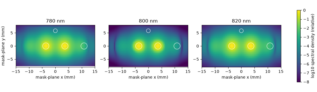
A column of physical wavevector \(\boldsymbol\kappa\) lands at \(\mathbf x=s(\omega)\boldsymbol\kappa\) in the mask plane. Drawn at three frequencies across the pulse’s spectrum, the exit field’s images stay where the achromatic tilt sends them, while each spot’s radius scales as \(1/\omega\) (by 5 % across these three): a fixed hole is a different cone of \(\boldsymbol\kappa\) at every frequency. The stored axes are in FFT order and the physical wavevector is their negative. Each column’s spectral energy is its squared field weighted by its real axial admittance in the sample, as every statistic here weights it.

field = output.plane_field(-1, convention="fft")  # (n_x*n_y, 1, n_omega)
power = np.real(exit_plane.admittance()) * np.abs(field[:, 0]) ** 2
kappa_x = np.fft.fftshift(-space.k_x)
kappa_y = np.fft.fftshift(-space.k_y)
figure, axes = plt.subplots(1, 3, figsize=(11, 3.2), layout="constrained")
for axis, wavelength in zip(axes, (780e-9, 800e-9, 820e-9), strict=True):
    index = int(np.argmin(np.abs(grid.omega - 2 * np.pi * C / wavelength)))
    scale = DISTANCE * C / grid.omega[index]
    image = np.fft.fftshift(power[:, index].reshape(space.n_y, space.n_x))
    view = axis.pcolormesh(
        scale * kappa_x * 1e3,
        scale * kappa_y * 1e3,
        np.log10(np.maximum(image / image.max(), 1e-8)),
        shading="auto",
        vmin=-8,
        vmax=0,
    )
    for (x0, y0), diameter in zip(centres, diameters, strict=True):
        axis.add_patch(
            Circle(
                (x0 * 1e3, y0 * 1e3), diameter * 1e3 / 2, fill=False, color="w", lw=0.8
            )
        )
    axis.set(
        xlim=(-15, 15),
        ylim=(-8, 8),
        aspect="equal",
        title=f"{wavelength * 1e9:.0f} nm",
        xlabel="mask-plane x (mm)",
    )
axes[0].set_ylabel("mask-plane y (mm)")
figure.colorbar(view, ax=axes, label="log10 spectral density (relative)", shrink=0.8)

<matplotlib.colorbar.Colorbar object at 0x71a0b1929940>

The colour spans eight decades. The signal, about \(10^{-3}\) of a beam, appears at \(3X\) and its mirror image \(2\mathbf k_2-\mathbf k_1\) at \(-3X\); each beam is wrapped in a faint halo from self- and cross-phase modulation; the dark hole sits clear of them all.

Along the sample

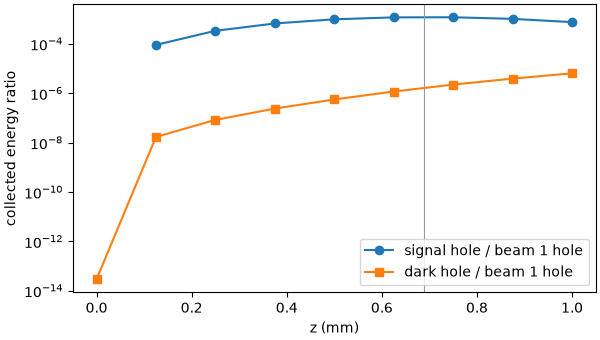
The statistics at every plane follow the signal as it grows. It does not grow steadily: in a dispersionless medium the signal wave’s longitudinal wavenumber misses the driving polarisation’s by \(\Delta k\approx-4K_0^2/k\), so the signal peaks near the coherence length \(\pi/|\Delta k|\) and falls back.

signal = collected[:, 2].sum(axis=-1) / collected[:, 0].sum(axis=-1)
dark = collected[:, 3].sum(axis=-1) / collected[:, 0].sum(axis=-1)
mismatch = 4 * K0**2 / (2 * np.pi * INDEX / WAVELENGTH)
print(f"coherence length pi/|dk| = {np.pi / mismatch * 1e3:.2f} mm")
print(f"signal peaks at z = {z[np.argmax(signal)] * 1e3:.3f} mm")
figure, axis = plt.subplots(figsize=(6, 3.4), layout="constrained")
axis.semilogy(z[1:] * 1e3, signal[1:], "o-", label="signal hole / beam 1 hole")
axis.semilogy(z * 1e3, dark, "s-", label="dark hole / beam 1 hole")
axis.axvline(np.pi / mismatch * 1e3, color="0.6", lw=0.8)
axis.set(xlabel="z (mm)", ylabel="collected energy ratio")
axis.legend()

coherence length pi/|dk| = 0.69 mm
signal peaks at z = 0.750 mm

<matplotlib.legend.Legend object at 0x71a0c8376900>

The dark hole reads \(3\times10^{-14}\) of beam 1’s hole at the entrance, the launch’s Gaussian tails, and grows only with the beams’ nonlinear halo. It is the diagnostic a dark corner gives: light there at the level of the signal would mean crosstalk – cubic products folded back by too coarse a grid, scattering from a collar, a beam wider than planned. Here it stays two decades below the signal, and halving the grid’s spacing in x or in y moves it by a few per cent only: it is physics, not the grid.

The chromatic weight

A hole centred on a Gaussian beam’s image collects

\[F=\int_0^\infty W(\rho)^p\,\frac{4\rho}{w_{ff}^2}\, e^{-2\rho^2/w_{ff}^2}\,d\rho,\]

with the far-field radius \(w_{ff}=2z_m/(kw_0)\) and \(k=\omega/c\), \(p=2\) under amplitude weighting and \(p=1\) under quadrature weighting (with \(W\) at the quadrature diameter). For a hard hole it is \(1-\exp[-D^2/(2w_{ff}^2)]\). The spot shrinks as frequency rises, so the hole collects more of the shorter wavelengths. At the entrance plane the beams are still Gaussian, so the integral is exact for the statistics’ paraxial map, up to the lattice.

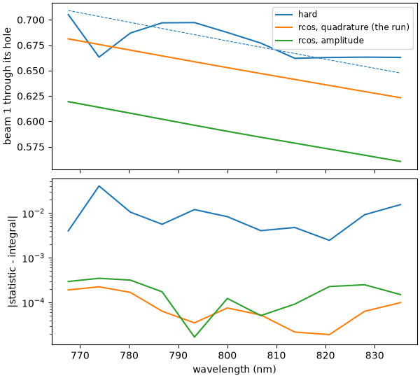
The run’s holes are raised cosines under quadrature weighting. The same launch, wrapped as a plane, goes through collect() with two other sets on the same centres: hard holes, and raised cosines under amplitude weighting.

def aperture_set(profile, weighting, edges=None):
    """The run's holes with another profile or weighting."""
    return ApertureSet(
        centres=centres,
        diameters=diameters,
        distances=[DISTANCE] * 4,
        edges=edges,
        profile=profile,
        weighting=weighting,
        labels=labels,
    )


def entrance_fraction(apertures):
    """Beam 1's collected fraction at the entrance through the first hole."""
    values = collect(
        StatsSpec(names=("beam_spectrum", "aperture_spectrum"), apertures=apertures),
        grid,
        SavedPlane(z=0.0, field=launch),
        flux=entrance,
    )
    # Equal beams: beam 1 carries half of the beam spectrum.
    return values["aperture_spectrum"][0][bright] / (
        0.5 * values["beam_spectrum"][bright]
    )


def exact_fraction(profile, weighting):
    """The integral F for the first hole, at each bright frequency."""
    width = float(np.asarray(holes.edges)[0]) if profile != "hard" else 0.0
    half = diameters[0] / 2
    if weighting == "quadrature":
        half = float(quadrature_half_width(half, width, profile))
    power_ = 1 if weighting == "quadrature" else 2
    values = []
    for w_ff in 2 * DISTANCE * C / (grid.omega[bright] * WAIST):
        value, _ = integrate.quad(
            lambda rho, w_ff=w_ff: (
                float(aperture_profile(rho, half, width, profile)) ** power_
                * 4
                * rho
                / w_ff**2
                * np.exp(-2 * rho**2 / w_ff**2)
            ),
            0.0,
            6 * w_ff + half + width,
            points=[half - width, half, half + width],
            limit=200,
        )
        values.append(value)
    return np.array(values)


rcos_edges = np.asarray(holes.edges)
cases = {
    "hard": (
        entrance_fraction(aperture_set("hard", "amplitude")),
        exact_fraction("hard", "amplitude"),
    ),
    "rcos, quadrature (the run)": (
        collected[0, 0][bright] / (0.5 * beam_spectrum[0][bright]),
        exact_fraction("rcos", "quadrature"),
    ),
    "rcos, amplitude": (
        entrance_fraction(aperture_set("rcos", "amplitude", edges=rcos_edges)),
        exact_fraction("rcos", "amplitude"),
    ),
}
hard_closed = cases["hard"][1]
wavelengths = 2 * np.pi * C / grid.omega[bright] * 1e9
order = np.argsort(wavelengths)
figure, (top, bottom) = plt.subplots(
    2, 1, figsize=(6, 5.4), sharex=True, layout="constrained"
)
for label, (statistic, exact) in cases.items():
    (line,) = top.plot(wavelengths[order], statistic[order], label=label)
    top.plot(wavelengths[order], exact[order], "--", color=line.get_color(), lw=0.8)
    lattice = np.abs(statistic - exact)
    bottom.semilogy(wavelengths[order], lattice[order], color=line.get_color())
    print(
        f"{label:>27}: lattice error <= {lattice.max():.1e}; "
        f"departure from the hard hole {np.max(np.abs(exact - hard_closed)):.1e}"
    )
top.set(ylabel="beam 1 through its hole")
top.legend(fontsize="small")
bottom.set(xlabel="wavelength (nm)", ylabel="|statistic - integral|")

                       hard: lattice error <= 4.0e-02; departure from the hard hole 0.0e+00
 rcos, quadrature (the run): lattice error <= 2.2e-04; departure from the hard hole 2.8e-02
            rcos, amplitude: lattice error <= 3.5e-04; departure from the hard hole 9.0e-02

[Text(0.5, 18.503588541666666, 'wavelength (nm)'), Text(25.503588541666673, 0.5, '|statistic - integral|')]

Solid lines are the statistics and dashed lines the integrals. The hard hole’s lattice error is a jagged staircase of a few per cent: on this lattice, six points across the far-field radius, columns step in and out of the hole as the frequency changes. The raised cosines, whose edge spans about two lattice spacings, follow their own integrals a hundred times more closely, to a few parts in \(10^{4}\) at the longest wavelengths, where the lattice is coarsest: a smooth weight converges on the lattice where a hard one does not.

What remains is each weighting’s departure from the hard hole, systematic and known. Under amplitude weighting the soft mask collects less than the hard hole by \(\int W(1-W)\) across its edge, at first order in the edge width: right for a physical soft mask, a bias as a stand-in for a hard one. Under quadrature weighting the edge’s area is corrected exactly, and only the slope of the intensity across the edge is left, \(\pi\sigma^2r\,\partial_\rho\bar I\) with \(\sigma^2=4m_2w^2\): a few per cent here, where the edge sits on the beam’s steepest part, and falling as \(w^2\) on a finer far-field lattice (a wider box), which admits a narrower edge.

A check on the kept plane

The exit plane’s field was kept, so its statistics can be recomputed from it. With collect, the same function a run uses, they agree to rounding. Written out from the definition – each column’s image at \(s\boldsymbol\kappa\), the profile at the quadrature diameter, the column’s admittance-weighted power summed – they agree too: on a Cartesian grid every column has the same transverse weight, so the ratio to the beam spectrum needs no further normalisation.

values = collect(
    StatsSpec(names=("beam_spectrum", "aperture_spectrum"), apertures=holes),
    grid,
    SavedPlane(z=LENGTH, field=field),
    flux=exit_plane,
)
difference = np.max(np.abs(values["aperture_spectrum"] - collected[-1]))
print(f"collect against the run: {difference / np.max(collected[-1]):.1e}")
columns_x, columns_y = (-axis.ravel() for axis in np.meshgrid(space.k_x, space.k_y))
by_hand = np.zeros((4, int(np.count_nonzero(bright))))
for hole_index, ((x0, y0), diameter, width) in enumerate(
    zip(centres, diameters, rcos_edges, strict=True)
):
    half = float(quadrature_half_width(diameter / 2, width, "rcos"))
    for column, index in enumerate(np.flatnonzero(bright)):
        scale = DISTANCE * C / grid.omega[index]
        rho = np.hypot(scale * columns_x - x0, scale * columns_y - y0)
        weight = aperture_profile(rho, half, width, "rcos")
        by_hand[hole_index, column] = np.sum(weight * power[:, index]) / np.sum(
            power[:, index]
        )
ratio = collected[-1][:, bright] / beam_spectrum[-1][bright]
print(
    "from the definition against the run, largest difference in collected fraction: "
    f"{np.max(np.abs(by_hand - ratio)):.1e}"
)

collect against the run: 2.5e-16
from the definition against the run, largest difference in collected fraction: 2.8e-16

Quadrants and the energy

The quadrants tile the columns exactly, so their sum is the beam spectrum to rounding. Beam 1 and the signal it feeds travel towards positive x, beam 2 and its signal towards negative x, and the two halves carry nearly equal energy. The boxes are half-open, so the column \(\kappa_x=0\) belongs to the positive side, and the row \(\kappa_y=0\), which carries the most energy, to the upper one: hence the upper quadrants’ larger share.

The beam spectrum weights each column by its real axial admittance in the sample, \(\varepsilon_0c^2\operatorname{Re}k_z/\omega\), about the index times \(\varepsilon_0c\) for these small angles: it is the physical axial flux inside the sample, and its integral over frequency is the energy statistic. The transmission of the exit face into air is not modelled.

regions = np.asarray(output["stats/region_spectrum"])[-1]
tiling = np.max(np.abs(regions.sum(axis=0) - beam_spectrum[-1]))
print(f"quadrants against the beam spectrum: {tiling / beam_spectrum[-1].max():.1e}")
quadrant_energy = regions.sum(axis=-1) * grid.d_omega
print(
    f"towards +x {quadrant_energy[1] + quadrant_energy[3]:.4e} J, "
    f"towards -x {quadrant_energy[0] + quadrant_energy[2]:.4e} J; "
    f"upper {quadrant_energy[2] + quadrant_energy[3]:.4e} J, "
    f"lower {quadrant_energy[0] + quadrant_energy[1]:.4e} J"
)
exit_energy = np.ravel(output["stats/energy"])[-1]
integral = np.sum(beam_spectrum[-1]) * grid.d_omega
print(
    f"exit energy {exit_energy:.6e} J; beam spectrum integral {integral:.6e} J; "
    f"relative difference {abs(integral / exit_energy - 1):.1e}"
)

quadrants against the beam spectrum: 4.8e-16
towards +x 1.3721e-07 J, towards -x 1.3708e-07 J; upper 1.5409e-07 J, lower 1.2020e-07 J
exit energy 2.742890e-07 J; beam spectrum integral 2.742890e-07 J; relative difference 0.0e+00

The absorbed power

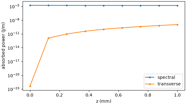
absorbed_power gives four powers in J/m, the spectral, transverse, evanescent and material channels; sampled at every step, their integral along z is the energy the absorbers took. The Kerr response moves energy between frequencies but adds none, so that integral matches the drop of energy from the entrance, to the trapezoid rule’s error over eight steps. The spectral channel, the absorption band, carries almost all of it; the transverse collar’s channel rises from nothing as the nonlinear halo creeps towards the grid’s edge, still more than four decades below; the evanescent and material channels are exactly zero.

rows_z = np.asarray(output["step_stats/z"])
rows = np.asarray(output["step_stats/absorbed_power"])  # (n_rows, 4)
at_entrance = np.asarray(output["stats/absorbed_power"])[0]
samples_z = np.concatenate([[0.0], rows_z])
samples = np.concatenate([at_entrance[None], rows])
absorbed = np.trapezoid(samples.sum(axis=1), samples_z)
energy = np.asarray(output["stats/energy"]).reshape(z.size, -1).sum(axis=1)
print(f"energy drop {energy[0] - energy[-1]:.4e} J; absorbed {absorbed:.4e} J")
figure, axis = plt.subplots(figsize=(6, 3.4), layout="constrained")
for channel, label in enumerate(("spectral", "transverse")):
    axis.semilogy(samples_z * 1e3, samples[:, channel], "o-", ms=3, label=label)
axis.set(xlabel="z (mm)", ylabel="absorbed power (J/m)")
axis.legend()
print(
    f"evanescent and material channels: {np.max(np.abs(samples[:, 2:])):.1f} J/m; "
    f"transverse at the exit {samples[-1, 1]:.1e} J/m"
)
print(f"tutorial run time: {time.perf_counter() - started:.1f} s")

energy drop 1.5701e-08 J; absorbed 1.5706e-08 J
evanescent and material channels: 0.0 J/m; transverse at the exit 1.1e-09 J/m
tutorial run time: 21.9 s

Related reading

Plane statistics defines the far-field statistics, their two weightings and what each backend computes; The free-space model gives the far-zone and Fourier-plane conditions and the paraxial error; Output: what a run leaves behind describes statistics-only planes. The design is SEP 23.