Nonlinear beam preparation and coupling into a capillary

A beam focused onto a gas-filled capillary often crosses some centimetres of the same gas first. When it is strong, the Kerr effect along that gap changes the beam before it reaches the entrance. This tutorial asks how much that changes the modes the capillary takes up. It propagates one physically focused beam through a 20 mm argon gap twice, once linearly and once with the Kerr effect. It takes each complete complex radial field at the entrance with field_plane(), couples it into the same capillary mode set with couple() under the scalar_paraxial model, and launches both through the same 5 mm Kerr-only capillary (Coupling simulations).

The system. A scalar, linearly polarised Gaussian at 800 nm, 30 fs intensity FWHM, on an envelope grid, in uniform argon at 3 bar and 293.15 K: the reference temperature of the argon polarisability, which the run records. The beam is built in the argon 20 mm before its linear focus, where its 1/e² intensity radius is 37.5 um. That focus is the entrance of a 75 um radius capillary (w/a = 0.5).

The model. Kerr self-focusing and self-phase modulation only (KerrResponse with thg=False). Plasma, third-harmonic generation and Raman scattering are omitted, in the gap and in the capillary. The ionisation they would carry is estimated offline at the end.

The strength. The energy is not a chosen number. It follows from the material functions and a target on-axis nonlinear phase of the linear Gaussian beam, \(B_{\rm lin} = 0.3\) rad, accumulated from the launch plane to the focus.

import math
import time

import matplotlib.pyplot as plt
import numpy as np
from scipy.special import j0, jn_zeros

from solprop import fourier
from solprop.constants import EPS0, C
from solprop.coupling import CouplingModel, couple
from solprop.driver import Simulation, SimulationSettings
from solprop.grid import EnvelopeGrid, RadialGrid
from solprop.modes.capillary import MarcatiliMode
from solprop.nonlinear.optmat_rates import OptmatRate
from solprop.nonlinear.responses import KerrResponse
from solprop.physdata import chi3, gamma3, refractive_index
from solprop.physdata.species import species
from solprop.processing import field_plane, get_spectral_density
from solprop.pulses import GaussianPulse, SpatialPulse
from solprop.spatial import SpatialMedium, critical_power
from solprop.stats import StatsSpec
from solprop.stepper import PIController

started = time.perf_counter()

The energy from the material functions

In the narrowband paraxial sizing model, a Gaussian of waist \(w_0\) in a medium of index \(n_0\) has Rayleigh length \(z_R = \pi n_0 w_0^2/\lambda_0\) and on-axis intensity \(I_0(z) = 2P_0/(\pi w_0^2[1+(z/z_R)^2])\). With the package’s scalar Kerr normalisation, \(n_2 = 3\chi^{(3)}/(4\varepsilon_0 c n_0^2)\). Integrating \(k_0 n_2 I_0\) from \(z = -L\) to the focus gives

\[B_{\rm lin} = \frac{2k_0 n_2 P_0 z_R}{\pi w_0^2}\arctan(L/z_R),\qquad U = P_0\,\tau_{\rm FWHM}\frac{\sqrt\pi}{2\sqrt{\ln 2}} .\]

\(n_0\) and \(\chi^{(3)}\) are optmat’s argon at 3 bar and 293.15 K. The energy is that of the beam through its launch plane, in the argon (Energy and flux in a medium).

WAVELENGTH = 800e-9  # m
FWHM = 30e-15  # s, intensity
PRESSURE = 3.0  # bar
GAP = 20e-3  # m, gas gap before the entrance
WAIST = 37.5e-6  # m, 1/e^2 intensity radius of the linear focus, at the entrance
RADIUS = 75e-6  # m, capillary core radius
LENGTH = 5e-3  # m, capillary segment
B_LINEAR = 0.3  # rad

medium = SpatialMedium("Ar", pressure=PRESSURE)
reference = species("Ar").susceptibility.reference_state.temperature
omega0 = 2 * math.pi * C / WAVELENGTH
n0 = float(refractive_index("Ar", omega0, pressure=PRESSURE))
susceptibility = chi3("Ar", pressure=PRESSURE, wavelength=WAVELENGTH)
n2 = 3 * susceptibility / (4 * EPS0 * C * n0**2)
k0 = 2 * math.pi / WAVELENGTH
rayleigh = math.pi * n0 * WAIST**2 / WAVELENGTH
peak_power = (
    B_LINEAR * math.pi * WAIST**2 / (2 * k0 * n2 * rayleigh * math.atan(GAP / rayleigh))
)
energy = peak_power * FWHM * math.sqrt(math.pi) / (2 * math.sqrt(math.log(2)))
critical = critical_power(WAVELENGTH, susceptibility, index=n0)
print(
    f"temperature {medium.temperature} K (argon polarisability reference {reference} K)"
)
print(f"n0 - 1 = {n0 - 1:.4e}, n2 = {n2:.4e} m^2/W, z_R = {rayleigh * 1e3:.3f} mm")
print(f"energy {energy * 1e6:.3f} uJ, peak power {peak_power * 1e-9:.4f} GW")
print(f"P0/Pcr = {peak_power / critical:.4f} (Pcr = {critical * 1e-9:.3f} GW)")

temperature 293.15 K (argon polarisability reference 293.15 K)
n0 - 1 = 7.7206e-04, n2 = 3.0931e-23 m^2/W, z_R = 5.527 mm
energy 12.114 uJ, peak power 0.3793 GW
P0/Pcr = 0.1238 (Pcr = 3.064 GW)

Two propagations through the gap

One SpatialPulse, focused 20 mm downstream (propz=-GAP) and built in the argon, starts both runs. The grids are the converged ones of the refinement study described at the end: 1 mm radial domain with 256 nodes, a 300 fs window over 500 nm to 1.4 um, and steps no longer than 0.25 mm. The only difference between the two runs is the response list.

grid = EnvelopeGrid.from_limits(GAP, WAVELENGTH, (500e-9, 1.4e-6), 300e-15, thg=False)
space = RadialGrid(1e-3, 256)
beam = SpatialPulse(
    GaussianPulse(wavelength=WAVELENGTH, fwhm=FWHM, energy=energy), WAIST, propz=-GAP
)
settings = SimulationSettings(
    controller=PIController(rtol=1e-7, atol=1e-14),
    save_planes=np.linspace(0, GAP, 41)[1:],
    dz_init=1e-5,
    dz_max=2.5e-4,
    stats=StatsSpec(names=("energy", "on_axis_intensity", "beam_radius")),
)
kerr = [KerrResponse(gamma3("Ar", wavelength=WAVELENGTH), thg=False)]
gap = {}
for name, responses in (("linear", []), ("Kerr", kerr)):
    simulation = Simulation.from_radial(
        grid, space, medium, responses, beam, settings=settings
    )
    gap[name] = (simulation, simulation.run(progress="none"))

The beam radius is the second moment of the time-integrated axial flux. The Kerr lens pulls the beam to a slightly smaller spot and moves its focus a little upstream. Its peak intensity rises by about 14 % but stays far from collapse.

figure, axes = plt.subplots(1, 2, figsize=(9, 3.5))
for name, (_, run) in gap.items():
    z = np.asarray(run["z"])
    radius = np.asarray(run["stats/beam_radius"])[..., 1].reshape(-1)
    intensity = np.asarray(run["stats/on_axis_intensity"]).reshape(-1)
    axes[0].plot(z * 1e3, radius * 1e6, label=name)
    axes[1].plot(z * 1e3, intensity * 1e-4, label=name)
axes[0].set(xlabel="z in the gap (mm)", ylabel="1/e² fluence radius (um)")
axes[1].set(xlabel="z in the gap (mm)", ylabel="on-axis peak intensity (W/cm²)")
axes[0].legend()
figure.tight_layout()
peak = {
    name: float(np.max(np.asarray(run["stats/on_axis_intensity"]))) * 1e-4
    for name, (_, run) in gap.items()
}
print(
    f"peak on-axis intensity: linear {peak['linear']:.3e}, "
    f"Kerr {peak['Kerr']:.3e} W/cm²"
)

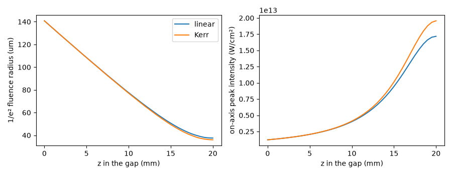
peak on-axis intensity: linear 1.717e+13, Kerr 1.956e+13 W/cm²

The fields at the entrance

field_plane(run, source=simulation) reads the last saved plane, the entrance, as a radial FieldPlane in the argon. Its columns are the Hankel spectrum of the field. The field anywhere in the plane is the inverse transform \(E(r) = \int k\tilde E(k)J_0(kr)\,dk\), so the field on the axis, which is not a radial node, is evaluated directly.

The wavefront change is the phase of the Kerr field relative to the linear one at the carrier frequency bin (800 nm), \(\arg[E_{\rm K}(r,\omega_0)/E_{\rm L}(r,\omega_0)]\). Both planes carry the same reference, because both runs share one frame. It is masked where the linear field’s amplitude at that bin falls below 1 % of its peak, where neither phase means much.

planes = {name: field_plane(run, source=sim) for name, (sim, run) in gap.items()}
hankel = space.hankel
r_plot = np.linspace(0, 150e-6, 301)
synthesis = j0(np.outer(r_plot, hankel.k_r)) * hankel.spectral_weights / (2 * math.pi)
centre = int(np.argmin(np.abs(grid.omega - grid.omega0)))
weights = fourier.energy_weights(grid.n_omega, grid.dt, kind=grid.kind)
admittance = n0 * EPS0 * C / 2
fields = {name: synthesis @ plane.samples[:, 0, :] for name, plane in planes.items()}
fluence = {
    name: admittance * np.sum(weights * np.abs(field) ** 2, axis=1)
    for name, field in fields.items()
}

figure, axes = plt.subplots(1, 2, figsize=(9, 3.5))
for name, values in fluence.items():
    axes[0].plot(r_plot * 1e6, values * 1e-4, label=name)
axes[0].axvline(RADIUS * 1e6, color="0.5", ls=":", label="core radius")
axes[0].set(xlabel="r (um)", ylabel="entrance fluence (J/cm²)")
axes[0].legend()
carrier = fields["linear"][:, centre]
resolved = np.abs(carrier) > 1e-2 * np.max(np.abs(carrier))
change = np.angle(fields["Kerr"][:, centre] / np.where(resolved, carrier, 1))
axes[1].plot(r_plot[resolved] * 1e6, change[resolved])
axes[1].axvline(RADIUS * 1e6, color="0.5", ls=":")
axes[1].set(
    xlim=(0, 150), xlabel="r (um)", ylabel="Kerr minus linear phase at 800 nm (rad)"
)
figure.tight_layout()
print(
    f"phase change at 800 nm: {change[0]:.3f} rad on axis, "
    f"{change[np.argmin(np.abs(r_plot - WAIST))]:.3f} rad at r = w0"
)

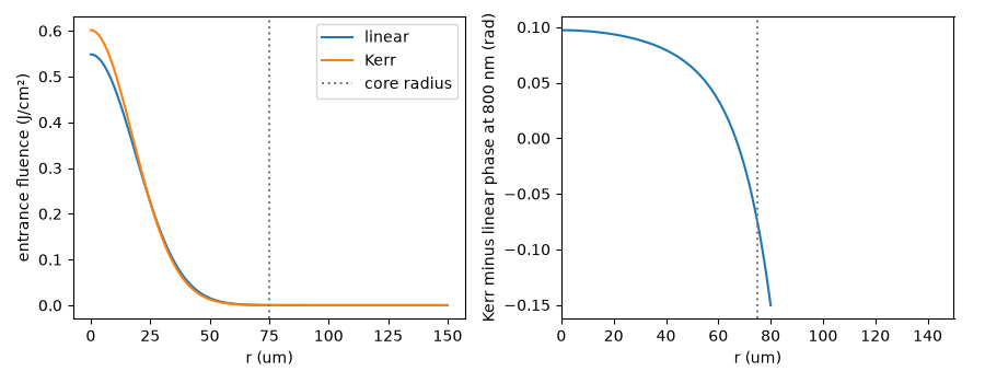
phase change at 800 nm: 0.097 rad on axis, 0.082 rad at r = w0

The fluence is the time integral of the axial flux, \(n_0\varepsilon_0c|E|^2/2\) summed over the spectrum (Energy and flux in a medium). The Kerr beam arrives about 10 % brighter on the axis and slightly narrower. At 800 nm it leads the linear field in phase by about 0.1 rad near the axis, and the lead falls away across the beam. That curvature is the Kerr lens: the beam is still converging as it reaches the entrance, while the linear beam is at its waist with a flat wavefront.

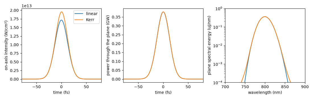
In time and frequency the changes are small. On the axis the pulse arrives brighter, and the power through the whole plane is unchanged, since the gap is lossless. The plane’s spectrum broadens a little by self-phase modulation, which shows only in its wings, three decades down.

t = grid.t
nodes = {
    name: fourier.inverse(
        fourier.spectrum_to_internal(plane.node_spectra()[:, 0, :], kind="envelope"),
        kind="envelope",
    )
    for name, plane in planes.items()
}
bin_width = 2 * math.pi / (grid.n_omega * grid.dt)

figure, axes = plt.subplots(1, 3, figsize=(11, 3.5))
for name, plane in planes.items():
    axis = fourier.inverse(
        fourier.spectrum_to_internal(fields[name][0], kind="envelope"), kind="envelope"
    )
    power = admittance * np.sum(
        hankel.radial_weights[:, None] * np.abs(nodes[name]) ** 2, axis=0
    )
    axes[0].plot(t * 1e15, admittance * np.abs(axis) ** 2 * 1e-4, label=name)
    axes[1].plot(t * 1e15, power * 1e-9, label=name)
    omega = plane.omega
    keep = omega > 0
    wavelength = 2 * math.pi * C / omega[keep]
    density = (
        plane.spectral_energy()[keep] / bin_width * omega[keep] ** 2 / (2 * math.pi * C)
    )
    sort = np.argsort(wavelength)
    axes[2].semilogy(wavelength[sort] * 1e9, density[sort] * 1e-9 * 1e6, label=name)
axes[0].set(xlim=(-80, 80), xlabel="time (fs)", ylabel="on-axis intensity (W/cm²)")
axes[0].legend()
axes[1].set(xlim=(-80, 80), xlabel="time (fs)", ylabel="power through the plane (GW)")
axes[2].set(
    xlim=(700, 900),
    ylim=(1e-4, 1),
    xlabel="wavelength (nm)",
    ylabel="plane spectral energy (uJ/nm)",
)
figure.tight_layout()

Coupling into the capillary

The receiving simulation is the 5 mm capillary on the same temporal grid, with eight \(HE_{1m}\) modes (the range of the recorded capillary envelope) and Kerr-only physics. Its input_port() describes the entrance. Each entrance plane is coupled under scalar_paraxial with an energy budget model_error = 0.05 for the approximation, its tails and its numerical errors (Coupling simulations). The launch is what the modes capture: nothing is rescaled.

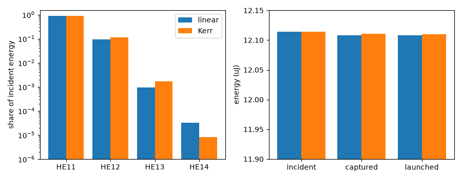
The modal share is \(s_m = U_m/U_{\rm incident}\): the energy launched into mode m, in its native true-power metric, over the incident energy of the whole entrance plane in the coupling’s common measure.

capillary = Simulation.from_capillary(
    RADIUS,
    LENGTH,
    "Ar",
    PRESSURE,
    lambda0=WAVELENGTH,
    grid=grid,
    envelope=True,
    fwhm=FWHM,
    energy=energy,
    modes=8,
    kerr=True,
    thg=False,
    plasma=False,
    raman=False,
    noise=None,
    n_save=21,
)
port = capillary.input_port()
model = CouplingModel("scalar_paraxial", model_error=0.05)
coupled = {name: couple(plane, port, model=model) for name, plane in planes.items()}
shares = {
    name: np.sum(weights * np.abs(result.launch.samples[:, 0, :]) ** 2, axis=1)
    / result.report.incident_energy
    for name, result in coupled.items()
}
print(coupled["Kerr"].report)
for name, result in coupled.items():
    report = result.report
    print(
        f"{name:>6}: s11 = {shares[name][0]:.5f}, s12 = {shares[name][1]:.5f}, "
        f"s13 = {shares[name][2]:.2e}; launched {report.efficiency:.5f} "
        f"of {report.incident_energy * 1e6:.3f} uJ; budget {report.budget:.3f}"
    )
delta = shares["Kerr"] - shares["linear"]
print(f"change: ds11 = {delta[0]:+.3e}, ds12 = {delta[1]:+.3e}, ds13 = {delta[2]:+.2e}")

CouplingReport: a field coupled into an input port
  model:          scalar_paraxial
  incident:       12.11 uJ
  launched:       12.11 uJ
  launched share: 0.9997 of the incident energy
  uncaptured:     3.36 nJ
  budget:         1.953e-02 of model_error 0.05
  angular:        6.250e-03 (field) incident field: cone-rule allocation (1 - cos the...
  numerical:      9.014e-28 (field) source content at the plane's spectral edge 9.0e-...
  target metric:  1.518e-03 (map) G (n_ref/Re n_eff) against the native identity
  angular:        1.024e-02 (map) retained target subspace: cone-rule allocation (1 -...
  source metric:  1.249e-05 (field) common measure M0 against the plane's native metric
  contrast:       n/a (model) not applied: a capillary wall is not a weakly guiding d...
  envelope:       1.503e-03 (model) capillary-he1m-scalar-vs-leaky-marcatili-2026-10
  passivity:      1.317e-08 (map) apparent gain within the model's defects, reported ...
  exterior:       zero
linear: s11 = 0.90618, s12 = 0.09229, s13 = 9.36e-04; launched 0.99953 of 12.114 uJ; budget 0.018
  Kerr: s11 = 0.88235, s12 = 0.11562, s13 = 1.68e-03; launched 0.99971 of 12.114 uJ; budget 0.020
change: ds11 = -2.383e-02, ds12 = +2.333e-02, ds13 = +7.40e-04

The Kerr-prepared beam puts 2.4 % of the incident energy less into \(HE_{11}\) and almost all of it into \(HE_{12}\). The total captured share barely moves: the change is a redistribution between modes, not a loss. The narrower, more curved entrance field looks more like the second mode.

labels = [f"HE1{m}" for m in range(1, 5)]
position = np.arange(4)
figure, axes = plt.subplots(1, 2, figsize=(9, 3.5))
for offset, name in ((-0.2, "linear"), (0.2, "Kerr")):
    axes[0].bar(position + offset, shares[name][:4], width=0.4, label=name)
    report = coupled[name].report
    axes[1].bar(
        np.arange(3) + offset,
        np.array(
            [report.incident_energy, report.captured_energy, report.launched_energy]
        )
        * 1e6,
        width=0.4,
        label=name,
    )
axes[0].set(
    yscale="log",
    ylim=(1e-6, 1.5),
    xticks=position,
    xticklabels=labels,
    ylabel="share of incident energy",
)
axes[1].set(
    xticks=range(3),
    xticklabels=["incident", "captured", "launched"],
    ylabel="energy (uJ)",
    ylim=(11.9, 12.15),
)
axes[0].legend()
figure.tight_layout()

The 5 mm capillary

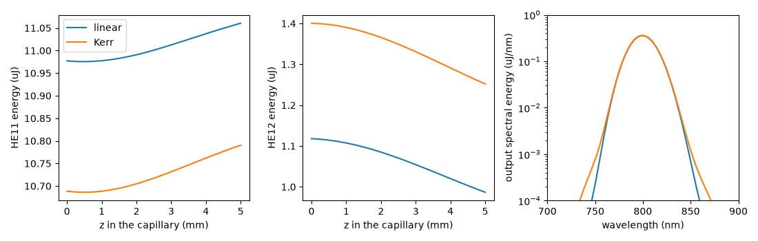
Both launches enter the identical capillary. Even linearly, \(HE_{11}\) and \(HE_{12}\) beat. With \(\beta_m \simeq nk_0 - u_m^2/(2nk_0a^2)\), where \(u_m\) is the m-th zero of \(J_0\), the beat length is

\[L_{\rm beat} = \frac{2\pi}{|\beta_{12}-\beta_{11}|} = \frac{8\pi^2 n a^2}{(u_{12}^2-u_{11}^2)\lambda_0} .\]

This is about 22.5 mm at the carrier, so the 5 mm segment holds about 0.22 beat periods. The output contains partial linear mode beating as well as modal filtering and the capillary’s own Kerr evolution. The capillary’s Marcatili modes below give the actual dispersive beat length, 19 to 28 mm across the pulse’s band, and the wall loss: over 5 mm, 0.2–0.5 % of \(HE_{11}\) and 1–2.4 % of \(HE_{12}\). Because both cases go through the same capillary physics, the beating, the loss and the Kerr coupling are the same in both. The difference between the outputs comes from the prepared incident field.

zeros = jn_zeros(0, 2)
carrier_beat = (
    8 * math.pi**2 * n0 * RADIUS**2 / ((zeros[1] ** 2 - zeros[0] ** 2) * WAVELENGTH)
)
print(
    f"carrier estimate: L_beat = {carrier_beat * 1e3:.2f} mm, "
    f"{LENGTH / carrier_beat:.3f} periods"
)
modes = [MarcatiliMode(RADIUS, "Ar", PRESSURE, kind="HE", n=1, m=m) for m in (1, 2)]
for wavelength in (650e-9, 800e-9, 950e-9):
    omega = np.array([2 * math.pi * C / wavelength])
    neff = [complex(mode.neff(omega)[0]) for mode in modes]
    beat = 2 * math.pi * C / (abs(neff[0].real - neff[1].real) * omega[0])
    alpha = [2 * value.imag * omega[0] / C for value in neff]
    print(
        f"{wavelength * 1e9:.0f} nm: L_beat = {beat * 1e3:.2f} mm; "
        f"power loss over 5 mm HE11 {1 - math.exp(-alpha[0] * LENGTH):.2e}, "
        f"HE12 {1 - math.exp(-alpha[1] * LENGTH):.2e}"
    )

outputs = {
    name: capillary.with_input(result.launch).run(progress="none")
    for name, result in coupled.items()
}
figure, axes = plt.subplots(1, 3, figsize=(11, 3.5))
for name, run in outputs.items():
    z = np.asarray(run["z"])
    modal = np.asarray(run["stats/energy"])[:, :, 0]
    axes[0].plot(z * 1e3, modal[:, 0] * 1e6, label=name)
    axes[1].plot(z * 1e3, modal[:, 1] * 1e6, label=name)
    wavelength, density = get_spectral_density(run, "wavelength", plane=-1, modes="sum")
    axes[2].semilogy(wavelength * 1e9, density * 1e-9 * 1e6, label=name)
    print(
        f"{name:>6} output: HE11 {modal[-1, 0] * 1e6:.4f} uJ, "
        f"HE12 {modal[-1, 1] * 1e6:.4f} uJ, "
        f"total {modal[-1].sum() * 1e6:.4f} uJ"
    )
axes[0].set(xlabel="z in the capillary (mm)", ylabel="HE11 energy (uJ)")
axes[1].set(xlabel="z in the capillary (mm)", ylabel="HE12 energy (uJ)")
axes[0].legend()
axes[2].set(
    xlim=(700, 900),
    ylim=(1e-4, 1),
    xlabel="wavelength (nm)",
    ylabel="output spectral energy (uJ/nm)",
)
figure.tight_layout()

carrier estimate: L_beat = 22.50 mm, 0.222 periods
650 nm: L_beat = 27.70 mm; power loss over 5 mm HE11 2.16e-03, HE12 1.13e-02
800 nm: L_beat = 22.50 mm; power loss over 5 mm HE11 3.27e-03, HE12 1.71e-02
950 nm: L_beat = 18.95 mm; power loss over 5 mm HE11 4.61e-03, HE12 2.41e-02
linear output: HE11 11.0604 uJ, HE12 0.9867 uJ, total 12.0529 uJ
  Kerr output: HE11 10.7903 uJ, HE12 1.2519 uJ, total 12.0511 uJ

In both cases \(HE_{12}\) gives energy to \(HE_{11}\) along the capillary, far more than its wall loss. Linear modes of a uniform capillary do not exchange energy, so this is the capillary’s Kerr coupling between the two modes. Its direction depends on their relative phase, which the partial beating advances. The Kerr-prepared launch leaves the capillary with about 0.27 uJ less in \(HE_{11}\) and 0.27 uJ more in \(HE_{12}\), close to the 0.29 uJ moved at the entrance.

Checks

Collapse, collar and aliasing. The peak power is an eighth of the critical power, and the peak intensity rises smoothly, so there is no collapse to resolve. The fluence in the outer tenth of the radial domain, the region next to the window, is printed below. So is the coupling’s numerical item, which measures the entrance planes’ content in the outer fifth of their transverse spectral window. Both are far below anything that could affect the shares.

for name, plane in planes.items():
    flux = admittance * np.sum(
        weights * np.abs(plane.node_spectra()[:, 0, :]) ** 2, axis=1
    )
    outer = space.r > 0.9 * space.radius
    collar = np.sum((flux * hankel.radial_weights)[outer]) / np.sum(
        flux * hankel.radial_weights
    )
    numerical = next(
        item for item in coupled[name].report.items if item.name == "numerical"
    )
    print(
        f"{name:>6}: outer-domain fluence {collar:.1e}, "
        f"spectral-edge content {numerical.value:.1e}"
    )

linear: outer-domain fluence 1.8e-30, spectral-edge content 6.8e-31
  Kerr: outer-domain fluence 3.5e-27, spectral-edge content 9.0e-28

Convergence. A separate refinement study varied the radial domain (0.8 to 1.5 mm), the radial nodes (192 to 512), the window (200 to 500 fs), the band (to 400 nm–2 um), the time step, the retained modes (4 to 8), the tolerance (1e-6 to 1e-9) and the maximum step (1 to 0.1 mm), one at a time. No variation moved \(s_{11}\) or \(s_{12}\) of either run by more than 3e-8. The combined uncertainty of the two runs is about 1e-6 of each change, far inside a tenth. An independent check projected each entrance field onto \(J_0(u_mr/a)\) with a Gauss–Legendre rule over the core. It agrees with couple to eight digits, once the captured share is converted to the launched share. The two differ by the ratio of the gas index to the mode index, about 8e-6.

Omitted ionisation. optmat’s recommended argon rate at 800 nm (OptmatRate) is integrated over the real field of a 30 fs Gaussian at the highest on-axis intensity of the Kerr run. This is an offline estimate, not part of the propagation.

rate = OptmatRate("Ar", WAVELENGTH)
times = np.linspace(-100e-15, 100e-15, 200001)
amplitude = math.sqrt(2 * peak["Kerr"] * 1e4 / (n0 * EPS0 * C))
envelope = amplitude * np.exp(-2 * math.log(2) * (times / FWHM) ** 2)
ionised = 1 - math.exp(
    -float(np.trapezoid(rate(envelope * np.cos(omega0 * times)), times))
)
electrons = ionised * float(medium.density(0.0))
plasma_index = electrons / (
    2 * EPS0 * 9.1093837139e-31 * omega0**2 / 1.602176634e-19**2
)
print(f"ionised fraction at {peak['Kerr']:.3e} W/cm²: {ionised:.1e}")
print(
    f"plasma index change {plasma_index:.1e} against Kerr {n2 * peak['Kerr'] * 1e4:.1e}"
)

ionised fraction at 1.956e+13 W/cm²: 1.1e-07
plasma index change 2.2e-09 against Kerr 6.1e-06

An ionised fraction of about 1e-7 lowers the index by about 2e-9. The Kerr index change it competes with is 6e-6. Leaving plasma out is defensible at this strength.

Energy meters. The energy here is the energy crossing the launch plane in the argon. A meter reading taken in air before a cell window is not that energy. Pass it through the window’s Fresnel transmission yourself, or transport the plane through a PlanarInterface, before giving it (Energy and flux in a medium, Coupling simulations).

print(f"run time {time.perf_counter() - started:.1f} s")

run time 9.7 s

Related reading

Coupling simulations describes planes, ports, coupling models and their budgets. The free-space model and Multimode capillaries: the coherent wall, tapers and gradients describe the two propagations. The design is SEP 31.