Generalised nonlinear Schrödinger propagation#
The generalised nonlinear Schrödinger equation (GNLSE) is the standard model of pulse propagation in a single-mode fibre: a dispersion \(\beta(\omega)\), a loss, a nonlinear coefficient \(\gamma\) and, optionally, a delayed Raman share \(f_R\). It describes a pulse envelope in a prescribed transverse mode. Use it when the effective area and propagation constant capture the spatial physics you need; it does not resolve redistribution of the field across a core or transfer to other modes. The N = 3 soliton lesson introduces dispersion, nonlinear phase, compression and recurrence with this model.
solprop represents this as a mode-averaged envelope calculation. A dispersion-specified mode supplies the propagation constant directly, and the coefficient mapping below converts \(\gamma\) into a third-order susceptibility. This makes the equation and its normalisation explicit when comparing it with field-resolved or multimode calculations.
This page is for users of prop_gnlse() who want to
know exactly which equation it integrates. It covers the fibre as a mode (including an
area and a dispersion that vary along the fibre), the mapping from \(\gamma\) to
\(\chi^{(3)}\) and why it reproduces the textbook equation, the shock term, the Raman
share, and the invariant the equation conserves. A run is one call:
from solprop.driver import prop_gnlse

output = prop_gnlse(
    0.11,  # gamma, 1/(W m)
    0.5,  # length, m
    [0.0, 0.0, -11.83e-27],  # beta_0, beta_1, beta_2 (s^2/m) about lambda0
    lambda0=835e-9,
    wavelength_limits=(500e-9, 2e-6),
    trange=4e-12,
    fwhm=50e-15,
    peak_power=1e3,
    pulseshape="sech",
    raman=True,  # fused silica, raman_fraction=0.2188 (optmat's bundle) by default
)
betas may be replaced by beta=(omega, beta) data or a callable, or by fibre= a
SpecifiedMode, any other Mode or a measured
IndexTable; loss_db_per_m sets a constant loss, shock (default True) the shock
term, and noise the shot noise (noise). The
soliton recurrence tutorial
runs an N-soliton through it.
The fibre is a mode#
solprop.nonlinear.gnlse.SpecifiedMode implements the whole
Mode protocol from
\(\beta(\omega)\) as a Taylor series about a reference frequency, \(\beta(\omega) = \sum_n \beta_n(\omega - \omega_\text{ref})^n / n!\), or as a table interpolated by a cubic spline;
a power loss, constant or a function of \(\omega\);
an effective area.
The effective index follows by inverting the definitions of conventions, §2,
and its frequency derivative is exact, taken in the polynomial or the spline basis, which
is what the co-moving frame needs: a finite-difference \(\beta_1\) would put a roughness
floor under the cumulative operator’s accuracy. The transverse profile is a uniform disc
whose area is the declared \(A_\text{eff}\) — the profile for which
\((\int|e|^2)^2/\int|e|^4\) is that area — so the single-node mode-averaged transform is
well defined and agrees with aeff. Because the mode is a full Mode, it enters the
modal transform like any other.
Two things it refuses. There is no effective index at or below zero frequency, where \(c\beta/\omega\) does not exist; asking for one raises rather than returning infinity, because the caller should be asking on the active band. And a table is never extrapolated: a spline or a high-order Taylor polynomial evaluated outside the data it was built from is the classic way to get a plausible, wrong answer. For the same reason there is no constructor that expands the series about zero frequency.
Loss is stated in dB/m at the interface and converted by
solprop.nonlinear.gnlse.attenuation_from_db():
\(\alpha = \ln(10)\,L/10\), so that the power falls as \(\mathrm{e}^{-\alpha z}\).
A varying effective area#
effective_area may be a ZProfile instead of a number,
which is how a taper reaches the GNLSE: aeff=Linear(1e-10, 2e-10, 0.1) in any of
the constructors, and prop_gnlse(..., fibre=...) unchanged. This is the
constant-dispersion special case: the dispersion and the loss stay functions of
frequency alone, which is exactly right for a fibre whose nonlinearity is
concentrated by a taper too weak to move its propagation constant, and it is the
case that keeps the compiled and device routes open, because the whole z dependence
is one scalar the cumulative operator can be expanded in. The next section is the
general case.
The area then enters exactly once, as the shape of the nonlinear coefficient.
The mode-averaged transform tabulates \(\sqrt{A_\text{eff}(0)/A_\text{eff}(z)}\) in
its taper_scale and the response prefactor keeps the entrance area, so the
propagated equation has
with the supplied \(\gamma\) as the entrance coefficient: only the area’s shape
is used, and a constant area cancels exactly. With n2 instead, the same holds
through \(\gamma = n_2\omega_0/(cA_\text{eff}(0))\). There is no second, absolute
division by an area anywhere, and no VaryingAreaGnlse: it is the same route.
\(A_\text{eff}(\omega, z)\) is not represented by one path. A frequency-dependent area is the declared reference-frequency slice \(A_\text{eff}(\omega_0, z)\) on this scalar route; a guide whose mode shapes genuinely depend on frequency is the business of the general modal route.
The declared path is the mode’s whole z dependence, so the fibre reports it as its
parameter_paths and its breakpoints are cross-section kinks: the transform’s area
and taper tables split on them, the cumulative operator makes them hard kinks, and
the schedule lands on them exactly. With no dispersion and no loss the phase is
\(P(t)\int_0^L\gamma(z)\,\mathrm{d}z\), which for a linear area is
\(\gamma\ln(1+\kappa L)/\kappa\), and the test suite checks the propagated phase against
it.
The fixed-step scaffold of solprop.driver.scaffold.propagate_fixed_rk4()
refuses a varying fibre: it evaluates the operator and the area once, at \(z = 0\).
A varying dispersion, declared with the area#
A real waveguide that tapers changes its propagation constant as well as its area: no guide has one without the other. So the dispersion may follow a path along z too, and when it does the area path is required beside it, declared at the same positions: a varying dispersion without a varying area, or the reverse, would be a silently inconsistent model.
solprop.nonlinear.gnlse.DispersionPath is the spectral sibling of
ZProfile. Where a ZProfile carries one scalar along the
fibre, a DispersionPath carries a whole frequency axis —
\(\beta(\omega, z)\), \(\partial\beta/\partial\omega(\omega, z)\) or
\(\alpha(\omega, z)\) — and answers the same four questions: where it kinks, what
interval it covers, whether it varies at all, and what its value is at a position.
Two implementations:
ConstantDispersionwraps a function of frequency alone, so the special case above is a path that never moves;InterpolatedDispersioncarries one ordinary dispersion per declared position and interpolates linearly between them, \(\beta(\omega, z) = (1-t)\beta_i(\omega) + t\beta_{i+1}(\omega)\) with \(t = (z - z_i)/(z_{i+1} - z_i)\).
Two constructors declare the pair together, which is what makes the model consistent:
from solprop.nonlinear.gnlse import SpecifiedMode

# One Taylor expansion set and one area per declared position.
fibre = SpecifiedMode.from_taylor_path(
    [[beta0, beta1_in, beta2_in], [beta0, beta1_out, beta2_out]],
    [0.0, 0.1],
    omega_ref=omega0,
    aeff=[1e-10, 0.6e-10],
)

# Or a measured n_eff(omega, z) table: its real part is beta and its imaginary
# part the loss, one row per position.
fibre = SpecifiedMode.from_index_path(
    omega, neff, [0.0, 0.05, 0.1], aeff=[1e-10, 0.8e-10, 0.6e-10]
)
SpecifiedMode.from_mode of a guide whose geometry moves — a capillary with a
tapered bore, a fibre on a pressure gradient — hands both over by itself: the
frozen callables forward the position to the source mode, and the area is sampled
from that same mode over the positions its own declared paths kink at. So
prop_gnlse(..., fibre=MarcatiliMode(Linear(...), ...), backend="numpy_ref") is a
run, not a refusal — with the backend named, for the reason the next paragraph
gives.
A provider channel’s area is taken at the pump. A general modal guide’s
ProviderChannelMode declares one surrogate area, the
scalar (∫|E|² dA)² / ∫|E|⁴ dA over the three components at the median knot of the
band the guide was sampled on — which is where the guide’s band is centred, not where the
pulse is. On the graded-index taper of the
moving solid guide worked example it
is 35 % above the pump’s. (This surrogate is what a mode-averaged interface means by an
area; it is not the channel’s nonlinear coefficient. Whether the longitudinal component
belongs in \(|E|^2\) here is an open question.) from_mode(channel, wavelength=...)
solves the channel’s area again
at that wavelength instead
(area_at()): once for a guide that does
not move, and at every sampled position of a moving guide’s path, so that a moving
channel hands over an area path at the pump beside its dispersion path. prop_gnlse
and Simulation.from_gnlse pass their lambda0, as they already read a table’s area
column there. A channel converted with neither aeff nor wavelength keeps the
median-knot surrogate and says so
(SurrogateAreaWarning). Every other mode’s area is not a
function of frequency in the Mode protocol, so wavelength is accepted and ignored
there.
The z dependence runs through one mechanism, the one a gas gradient runs
through. The declared positions are the cumulative operator’s hard kinks, so the
adaptive Chebyshev split never straddles a corner and the schedule lands on it; a
linearly interpolated path is degree one in \(z\) between corners, so the operator is
resolved exactly there and its integral is exact too. What changes against the
constant-dispersion case is the representation: a mode whose dispersion moves is
not a function of one scalar parameter, so build_phi tabulates the operator
along \(z\) instead of expanding it in parameters — the general representation. Every
CPU backend evaluates that table: numpy_ref and numba_cpu on the host, and the
native backend’s CPU build in its own kernels, so the default backend="auto" runs a
moving-dispersion fibre (Varying operators and interpolation accuracy). The native backend’s GPU
builds refuse the table by name, since they would hold it on the device; run such a
fibre on a CPU build there. The area-only case above keeps its one-parameter
expansion, and every backend with it.
One consequence of how InterpolatedDispersion answers “do I move?”: it compares
its declared sets by identity, so a path whose positions carry equal but
distinct objects reads as moving. Declaring the same TaylorDispersion twice is a
fibre that does not move; declaring two identical ones is a fibre that takes the z
table and loses the GPU route with it. Pass the same object, or a plain function
of frequency, when nothing is meant to change.
The closed form this is measured against is the walk-off of a linear \(\beta_1\) path. In a frame with \(\beta_1\) pinned at the entrance, \(D(\omega, z) = -\mathrm{i}\,(\beta_1(z) - \beta_1(0))(\omega - \omega_0)\), so \(\Phi\) is a pure delay of \(\int_0^Z (\beta_1(z) - \beta_1(0))\,\mathrm{d}z\), which is \(gZ^2/2\) for \(\beta_1(z) = \beta_1(0) + gz\). It is reproduced to 6.1e-13 relative, which is the round-off of the cancellation inside \(D\) and not an interpolation error.
Four things are refused by name rather than approximated: a declared path whose positions do not cover the run — the value, the derivative and the loss are each checked, because any of them would otherwise carry its last value silently over the rest of the fibre; a dispersion path without an area path beside it; a value and a derivative that disagree about whether they move; and an area path declared at other positions than the spectral paths that move. Those positions are the union over the value, the derivative and the loss, so a fibre whose attenuation alone follows a path is a fibre like any other — it declares its area at the loss’s positions — and a corner declared in one path alone is a corner the schedule still lands on, because the area path carries it. An \(n_\text{eff}\) table that does not span the active band is refused by the same no-extrapolation rule as any other table.
The coefficient mapping#
solprop.nonlinear.gnlse.problem_from() performs the mapping
The factor \((1 - f_R)\) is applied with raman=True, or with Raman off when a
raman_fraction is given (below).
\(A_\text{eff}\) is one unless a real area is given, which is the usual GNLSE convention:
the area has already been folded into \(\gamma\). The \(4/3\) undoes the \(3/4\) of the envelope
Kerr response, and the linear index in the \(n_2 \leftrightarrow \chi^{(3)}\) conversion is
taken as one, consistently with the prefactor below.
The normalisation prefactor uses \(n_\text{eff} = 1\) rather than \(c\beta/\omega\). That is
not an approximation but a statement about what a GNLSE \(\beta\) is: a fitted dispersion
relation, which carries the whole of the waveguide and the material and need not be
anywhere near a physical effective index — it is routinely written with \(\beta_0 = 0\), at
which \(c\beta/\omega\) vanishes. solprop records the choice on the problem as
prefactor_index, so that a consumer does not have to know it by folklore.
It comes out as the textbook equation#
Put the chain together for a continuous wave, where the spectrum is a single bin and no transform is involved. With \(E = A\,/\sqrt{\varepsilon_0 c A_\text{eff}/2}\) and \(P = \tfrac34\varepsilon_0\chi^{(3)}|E|^2E\),
which at \(\omega = \omega_\text{ref}\) is \(-\mathrm{i}\gamma|A|^2A\): the GNLSE, with the sign the internal FFT convention gives it, and with the shock factor \(\omega/\omega_0\) already in place. In the optics convention of the user interface the same equation reads \(+\mathrm{i}\gamma|A|^2A\) (conventions, §2). This identity is asserted directly by the test suite, on both grids, which is the tightest available check that the mapping, the response and the prefactor agree with one another.
The shock term#
shock=True is the \(\omega\) dependence of the prefactor and nothing else; shock=False
freezes its numerator at \(\omega_\text{ref}\). There is no time-domain derivative and no
\(1/\omega\) to guard against, because the prefactor is only evaluated on the active band.
Three frequency dependences are easily confused here, and they are separate:
The UPPE frequency factor, the \(\omega\) of the prefactor: a property of the output frequency of the polarisation, which
shockswitches. In the envelope limit it gives self-steepening.Modal dispersion of the nonlinearity: a frequency-dependent effective area or overlap, a geometric property of the guide. This route holds the area at the reference frequency (a varying effective area); the general modal route carries mode shapes that depend on frequency.
Material dispersion of \(\chi^{(3)}\): the susceptibility’s dependence on all four frequencies of each quartet, which neither of the others supplies. A GNLSE’s \(\gamma\) is one fitted constant, so this route has none, and it refuses the dispersive electronic policies of a gas run (a frequency-dependent electronic response).
The Raman fraction is not silently taken#
\(f_R\) reserves a share of \(\gamma\) for a Raman response. raman_fraction defaults to
None, which is silica’s \(f_R\) with raman=True — 0.2188, the fraction of optmat’s
silica bundle (below) — and \(f_R = 0\) with Raman off,
so by default solprop gives the whole of \(\gamma\) to the Kerr term when there is no
Raman response: prop_gnlse defaults to raman=False, and then the \((1 - f_R)\) factor
is not applied. Were the silica fraction reserved regardless, the default would
propagate 78 % of the nonlinearity asked for, and an “N = 6” soliton would really be
\(N = 5.30\) and would not recur.
That default is the textbook “no Raman”: \(f_R = 0\) at fixed \(\gamma\), the whole response
treated as instantaneous. A pair of runs that switches only raman then keeps \(N\), the
nonlinear length and the long-pulse self-phase modulation, and differs by the delay of
the response alone. The other counterfactual — the delayed part of the material removed,
the instantaneous part left as it was, which is Luna’s prop_gnlse — is the same pair
of runs with the fraction given explicitly: raman_fraction passed with raman=False
is always held back, so raman=False, raman_fraction=0.2188 propagates
\(0.7812\,\gamma\) as Kerr and nothing else, and switching on raman adds the Raman response to exactly that
Kerr term. The problem records the fraction that was held back as raman_fraction,
whether or not a response carries it.
With raman=True the share is taken and given to a response: the mapping declares a
fused-silica RamanResponse beside the reduced Kerr term,
and the two together carry the whole of \(\gamma\). The two susceptibilities are not the
same number for the same share, because the envelope forms differ — the Raman drive carries
a half where the envelope cubic carries three quarters — so a Raman term of integral \(X\)
acts like a Kerr term of \(\tfrac23X\) and
which is solprop.nonlinear.gnlse.raman_susceptibility() times \(f_R\). The identity
\(\tfrac23 f_R X_\text{full} + \chi^{(3)}_\text{Kerr}(f_R) = \chi^{(3)}_\text{total}\)
holds by construction and is a test, and the split itself is
solprop.nonlinear.gnlse.kerr_susceptibility(). The Raman page derives the
factors and lists what the physics tests pin.
Fused silica’s response comes from optmat’s silica bundle
(materials), under the default
selection (materials=None, which is MaterialSelection()) as under any other. The rule
above, with the bundle’s numbers:
|
|
held back from Kerr |
the Raman response |
|---|---|---|---|
on |
|
the bundle’s \(f_R\): 0.2188 for the default bundle |
the bundle’s \(h_R\), carrying \(f_R\) |
off |
|
0: the whole of \(\gamma\) is Kerr |
none |
on |
given |
the given fraction |
the bundle’s \(h_R\), carrying it |
off |
given |
the given fraction |
none |
The bundle’s \(f_R\) is the one optmat’s Kerr fit found with Hollenbeck and Cantrell’s
shape, so the pair is consistent with the fit’s total \(n_2\), which
n2="recommended" takes at the carrier lambda0 (it needs a fibre with an area, as
any n2 does); a given gamma or n2 sets the total, and the bundle’s fraction
splits it unless one is given. materials=MaterialSelection(raman="tensor") takes Lin
and Agrawal’s bundle instead, with its own \(f_R = 0.245\) and its copolarised
\(a + b\); another name is any optmat silica bundle’s. The response is the bundle’s
normalised shape sampled into one undamped row with no dephasing
(SampledShape), at the amplitude
raman_susceptibility() above. optmat’s own silica
raman_coefficient and electronic_susceptibility include its \(n_0^2 \approx 2.1\),
which this mapping’s \(n_0 = 1\) does not, so they are never imported. The run’s
material manifest records the fraction held back and where it came from — "bundle",
"user", or "raman-off" — with the bundle and the origin of \(n_2\).
Which invariant the equation has#
A lossless fibre with the shock term on conserves photon number,
\(\sum_k|\tilde A(\omega_k)|^2/\omega_k\), and not energy: the Raman response moves photons
down in frequency and each one carries away less energy than it brought. Measured over a
hundredth of a soliton period with a given \(f_R = 0.18\), the photon number is conserved exactly and
the energy falls by \(7.2\times10^{-6}\). With shock=False the prefactor is frozen at the
carrier and the equation conserves energy instead, which is the wrong invariant for a
delayed response; with Raman off both hold to \(5.6\times10^{-16}\).
A worked example#
A soliton in a silica-like fibre: the mapping, and the soliton order it implies.
import matplotlib.pyplot as plt
import numpy as np

from solprop.constants import C
from solprop.grid import EnvelopeGrid
from solprop.linear import Frame, dispersion_operator
from solprop.nonlinear.gnlse import problem_from

grid = EnvelopeGrid.from_limits(1.0, 835e-9, (500e-9, 2e-6), 12.5e-12)
beta2 = -11.83e-27           # s^2/m, anomalous
problem = problem_from(
    [0.0, 0.0, beta2], omega_ref=grid.omega0, gamma=0.11, aeff=1.0
)

duration = 28.4e-15          # sech half-width
orders = np.arange(1, 7)
peak = orders ** 2 * abs(beta2) / (problem.gamma * duration ** 2)

operator = dispersion_operator(problem.mode, grid, Frame.comoving(grid))
active = grid.active_mask
omega = grid.omega[active]
order = np.argsort(omega)

fig, (left, right) = plt.subplots(1, 2, figsize=(7.0, 3.0), layout="constrained")
left.plot(1e-12 * (omega[order] - grid.omega0) / (2 * np.pi),
          -np.imag(operator)[active][order],
          lw=1.6, color="C0")
left.set_xlabel(r"$(\omega - \omega_0)/2\pi$  (THz)")
left.set_ylabel(r"$-\mathrm{Im}\,D$  (1/m)")
left.set_title("the fibre's dispersion in the frame")

right.semilogy(orders, peak, "o-", lw=1.4, color="C1")
right.set_xlabel("soliton order $N$")
right.set_ylabel("peak power (W)")
right.set_title(r"$P_0 = N^2 |\beta_2| / (\gamma \tau^2)$")
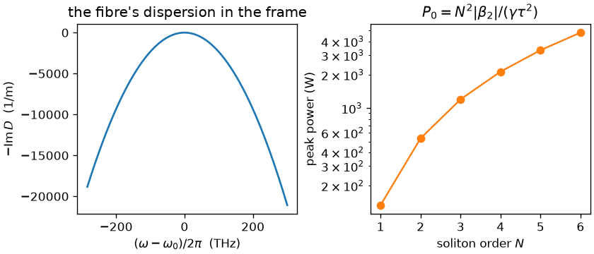
The operator is a pure parabola, because the fibre was given only \(\beta_2\) and the frame removed the rest. The N = 6 case on the right is the classic soliton-recurrence test: with Raman off, an exact higher-order soliton returns to its input shape after one soliton period, which checks the dispersion, the Kerr term and the mapping together.