9. Raman scattering#
The Kerr effect is instantaneous on the time scale of an optical pulse, because bound electrons respond within a fraction of a femtosecond. Molecules and glasses also have a slower response. The light sets nuclei in motion, either rotating a molecule or stretching a bond, and that motion changes the polarisability seen by later light. The medium remembers the pulse. In a fibre this delayed response produces the soliton self-frequency shift and Raman gain. In a gas-filled fibre it produces rotational and vibrational Raman frequency combs, impulsive excitation and long-lived molecular coherences, which can couple successive pulses.
This chapter explains how solprop writes that memory: as a causal convolution, with a response function whose units, normalisation and sign are fixed once. It covers the physical origin of the response, the models for gases and for silica, the factor of \(\tfrac23\) that separates a Raman share at the level of the field from one at the level of the envelope, which sign of the response means gain, the vector response, and how the convolution is computed.
9.1 The response function#
For a fixed linear polarisation in an isotropic medium, solprop writes the Raman polarisation as
(the response function and its units), with \(\rho\) the number density. Causality is the upper limit, and \(h(t)=0\) for \(t\le0\). The dimensions fix \([h]={\rm m^5V^{-2}s^{-1}}\), so \(\int h\,\mathrm dt\) has the units of the per-particle Kerr coefficient. A Raman fraction is then a share of the same quantity. The drive \(E^2\) is the real field squared. The molecule responds to the intensity, not to the oscillating field, and the response multiplies the field again.
This convention is linear in \(\varepsilon_0\). Some codes, including Luna, write the same physics with \((4\pi\varepsilon_0)^2\) inside every scale factor and no \(\varepsilon_0\) outside, so their \(h\) is quadratic in \(\varepsilon_0\). Converting between the two divides by \(\varepsilon_0\), and mixing them is a factor of \(10^{11}\) error that is hard to miss but easy to make.
9.2 Where the response comes from#
An induced dipole in a field has interaction energy \(U=-\tfrac12E_i\alpha_{ij}E_j\). The half matters, because the dipole is induced and grows as the field is applied. For a linear molecule with orientation \(\mathbf n\), the polarisability tensor is \(\alpha_{ij}=\bar\alpha\delta_{ij}+\Delta\alpha(n_in_j-\delta_{ij}/3)\) (physical origin).
Vibration. The mean polarisability depends on the bond length \(q\), so the field exerts a force \((\partial\bar\alpha/\partial q)E^2/2\) on the vibrational coordinate. The displacement then changes the polarisation through the same derivative, so the vibrational strength carries \((\partial\bar\alpha/\partial q)^2\).
Rotation. The anisotropy \(\Delta\alpha\) produces a torque that aligns the molecule with the field. The aligned ensemble has a different refractive index for later light. Quantum mechanically this is a ladder of rotational Raman transitions, \(J\to J+2\).
Two clocks matter: the molecular period \(2\pi/\Omega\) and the coherence decay time \(\tau_2\) (steady-state, transient and impulsive regimes). If a nearly monochromatic pump and Stokes field beat for many decay times, the result is steady-state stimulated scattering with a Lorentzian gain. If the pulse is shorter than \(\tau_2\) but longer than the period, the scattering is transient. If the pulse is shorter than a molecular period, it excites the molecule impulsively and leaves it ringing, and later light samples that ringing. Comparing the pulse duration with \(\tau_2\) alone does not distinguish the last two cases. The same causal convolution describes all three, within its assumptions of weak excitation of an initially isotropic ensemble. Strong alignment or significant population transfer would need a different model.
9.3 Models#
The building block is the damped oscillator,
with integral \(K\Omega/(\Omega^2+\tau_2^{-2})\) (the damped oscillator). Kolesik and Moloney (2014, Eq. 56) and Couairon et al. (2011, Eq. 121) use the same normalisation. solprop’s models for gases are sums of such lines, with their strengths derived from molecular data:
Vibrational modes have \(K=(4\pi\varepsilon_0\,\partial\alpha/\partial Q)^2/(2\mu\Omega_v\varepsilon_0)\), where the \(4\pi\varepsilon_0\) converts a tabulated volume polarisability derivative to SI. Luna’s denominator is \(4\mu\Omega\), so its vibrational amplitude is half of solprop’s. solprop’s guide explains why the factor of 2 is not doubled (the vibrational mode).
Rotational ladders sum the S-branch lines \(J\to J+2\), each weighted by the difference of the thermal populations of its two levels,
\[ K\frac{(J+1)(J+2)}{2J+3}\Big(\frac{p_{J+2}}{2J+5}-\frac{p_J}{2J+1}\Big),\qquad K=-\frac{(4\pi\varepsilon_0)^2}{\varepsilon_0}\frac{2}{15}\frac{\Delta\alpha^2}{\hbar} \]
For the built-in molecular gases, optmat supplies the whole response: lines, strengths, and widths that depend on density and on the collision partners (Raman data and validity). Nitrogen at room temperature has 106 lines in 43 damping groups. In air its lines are broadened by nitrogen, oxygen and argon separately, not by “the total density”. The rotational revival period of a molecule is \(1/(2Bc)\), which gives 8.4 ps for nitrogen and 0.28 ps for hydrogen. A hydrogen rotational coherence at 1 bar lives for nanoseconds, far longer than a typical simulation window.
Fused silica has no discrete molecular lines but a broad amorphous band. The classic model is the single damped oscillator of Blow and Wood (1989), with time constants of 12.2 fs and 32 fs. Stolen et al. (1989) derived the response from the measured Raman gain. Hollenbeck and Cantrell (2002) fitted thirteen intermediately broadened modes to the gain spectrum. Lin and Agrawal (2006) added the “boson peak” and an anisotropic part. solprop takes silica’s response from optmat’s bundles, which hold the total \(n_2(\lambda)\), a response shape of unit integral and that shape’s own Raman fraction together, so that they cannot be mismatched (fused silica’s nonlinear response):
bundle |
shape |
\(f_R\) |
|---|---|---|
default |
Hollenbeck and Cantrell (2002), with optmat’s Kerr fit |
0.2188 |
tensor |
Lin and Agrawal (2006), isotropic \(a\) and anisotropic \(b\) |
0.245 |
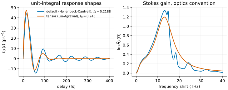
Fused silica’s two response shapes, each of unit integral, and the imaginary parts of their
spectra, which are the Raman gain on the Stokes side in the optics convention. Computed from
solprop’s SilicaBundle by docs/primer/figures/primer_figures.py.#
The literature’s values of \(f_R\) differ partly because they define it differently:
0.18, from Stolen et al. (1989), was estimated from Hellwarth, Cherlow and Yang (1975) and Stolen and Ippen (1973). Hollenbeck and Cantrell and Dudley, Genty and Coen use it.
0.21 ± 0.03 is Hellwarth, Cherlow and Yang’s nuclear share.
0.222 is the envelope share implied by Blow and Wood’s field-level weights.
0.245 is Lin and Agrawal’s, chosen to reproduce the measured peak gain.
Watch the letter \(\alpha\) in this literature: in Blow and Wood it is the Kerr share, 0.7, and in Stolen et al. it is the Raman share, 0.18.
9.4 The two-thirds, and the Raman fraction#
On an envelope grid, the cycle-averaged drive is \(E^2\to\tfrac12|A|^2\), whereas the Kerr cubic gives \(\tfrac34|A|^2A\). A Raman term whose kernel integrates to \(X\) therefore produces the same long-pulse nonlinear index as a Kerr term of \(\tfrac23X\). Blow and Wood (1989, after Eq. 8) note the same factor: their envelope kernel is \(\alpha\delta(t)+\tfrac23(1-\alpha)g_R(t)\), and “the 2/3 factor arises from neglecting a cross term”. So if a share \(f_R\) of the total nonlinearity is to be Raman, the per-particle kernel must satisfy
while the Kerr term keeps \((1-f_R)\) of the total. On the GNLSE route, which works with an effective kernel at density one and unit index,
this reads \(\int h\,\mathrm dt=\tfrac32f_R\chi^{(3)}_{\rm total}=2f_Rn_2\varepsilon_0c\) (Chapter 3). The identity
\(\tfrac23\cdot\tfrac32f_R+(1-f_R)=1\) is built into solprop’s mapping and tested
(Raman in a fibre GNLSE). \(f_R\) is therefore an
envelope quantity: a share of the cycle-averaged nonlinear index. Some reviews put one share on
both the field-level cubic and the field-level drive, which gives a different envelope share. Chapter
3 explains what raman=False means on the GNLSE route.
9.5 Which sign is gain#
The Raman gain lives in the imaginary part of the response’s spectrum. In the optics convention of this primer, with \(\tilde H(\Omega)=\int_0^\infty h(\tau)e^{+i\Omega\tau}\mathrm d\tau\), the damped oscillator has \(\operatorname{Im}\tilde H(\Omega)>0\) near its resonance, and that is gain on the Stokes side. optmat, Stolen et al., Hellwarth et al. and Lin and Agrawal use this convention (Blow and Wood 1989, Eq. 3, use the opposite sign), so the Stokes gain is \(g\propto\omega_s\rho\operatorname{Im}\tilde H(\Omega)\) (the sign that means gain). Inside solprop the kernel is transformed with the FFT sign, so there \(\operatorname{Im}\tilde H<0\) is gain. The kernel is an internal array and must never be passed through the convention conversion: conjugating it would silently exchange the Stokes and anti-Stokes sides.
9.6 The vector response#
Two polarisation components see a Raman medium differently, because the rotational response aligns molecules along the field. Averaging over the orientations of an isotropic ensemble gives two channels. The vibrational (isotropic) channel responds to the trace of \(Q=\mathbf E\mathbf E^T\). The rotational (anisotropic) channel responds to its traceless part:
(the vector response). This is the same decomposition as Hellwarth’s isotropic and anisotropic kernels \(a(t)\) and \(b(t)\) (Hellwarth, Cherlow and Yang 1975, Eq. 2), and it is how Lin and Agrawal (2006, Eq. 1) write silica’s tensor. Two results follow. A probe polarised across the pump sees the rotational response with \(-\tfrac12\) of its parallel strength. At equal power, a fixed circular envelope has a quarter of the rotational source of a linear one and the same vibrational source. That is a statement about the source, not a gain ratio: a Stokes wave of the opposite helicity couples through the remaining term of the response, so the rotational Raman gain does not simply fall by four (scalar reduction, rotations and circular coordinates). The orientation average is three-dimensional even when only two transverse components are propagated.
9.7 Computing the convolution#
solprop evaluates the convolution with FFTs (how the convolution is evaluated). Two details matter. The drive is padded onto a grid twice as long, so that the circular convolution of the FFT becomes the linear, causal one. Without the padding, a molecular coherence that outlives the window would wrap around and act on the leading edge of the pulse. The kernel tail is tapered over the grid’s collar width. Each damping group is also dephased separately: summing a rotational and a vibrational response and damping the sum once would be wrong.
The drive depends on the grid: \(E^2\) on a field grid with the harmonic, \(\tfrac12|E_a|^2\) without it, and \(\tfrac12|A|^2\) on an envelope grid (the drive, and why it differs between the grids). Kolesik and Moloney (2014, §3.1.4) suggest integrating the oscillator equation along the time axis instead, which is cheaper for one or two lines. solprop’s gas responses carry tens of damping groups and nanosecond coherences, which is why it convolves instead.
The window has to contain what the measurement depends on. A pulse resolved in a 1 ps window says nothing about a molecular coherence that persists for nanoseconds and acts on the next pulse. That physics needs a window covering it, or a model that carries the coherence between pulses.
What to remember
\(P=\varepsilon_0\rho E\int h(t-t')E^2(t')\,\mathrm dt'\), with \(h\) linear in \(\varepsilon_0\) and in m⁵V⁻²s⁻¹. Luna’s convention is quadratic in \(\varepsilon_0\).
Vibration couples through \(\partial\bar\alpha/\partial q\), rotation through \(\Delta\alpha\). The pulse duration against the period and against \(\tau_2\) decides the regime.
Gas responses come from optmat as sums of damped lines with partner-resolved widths. Silica comes as a bundle of \(n_2\), shape and \(f_R\): 0.2188 by default, 0.245 for the tensor.
On an envelope, a Raman kernel of integral \(X\) acts like Kerr \(\tfrac23X\), so \(\rho\int h=\tfrac32f_R\chi^{(3)}_{\rm total}\). \(f_R\) is an envelope share.
In the optics convention, \(\operatorname{Im}\tilde H>0\) is Stokes gain. Internally the sign is the opposite, and the kernel is never converted.
The vector response has an isotropic and a traceless channel. At equal power a fixed circular envelope has a quarter of the linear rotational source; that is not a gain ratio.
The convolution is linear on a doubled grid. The window must contain the coherence the result depends on.
The precise statements are in the Raman response, Raman response models, polarisation-dependent Raman response, evaluating a Raman response and Raman data and validity. Chapter 10 frees the electrons.