2. The unidirectional pulse propagation equation#
Chapter 1 ended with a second-order equation in \(z\) for each frequency and transverse label. A second-order equation in \(z\) needs two boundary conditions: the field and its derivative, or equivalently the light entering from both ends. That is not the problem you want to solve. You know the pulse at the entrance and want it downstream, and almost nothing travels backwards. This chapter shows how to make that intuition exact. The second-order equation is split into an exact pair of first-order equations, one for the forward wave and one for the backward wave. Then one approximation is made, which removes the backward wave.
The result is the unidirectional pulse propagation equation (UPPE) of Kolesik, Moloney and Mlejnek (2002) and Kolesik and Moloney (2004). solprop solves this equation in all its routes. The chapter covers what the approximation costs, where the self-steepening and space-time-focusing terms come from, what the moving frame does and does not change, and why an envelope equation is not, by itself, an approximation. It ends with the equation exactly as solprop states it.
2.1 Forward and backward waves#
Start from the scalar, transversely transformed wave equation of §1.5, with the current absorbed into an equivalent polarisation \(\tilde P\to\tilde P+i\tilde J/\omega\) (which reproduces the \(-i\mu_0\omega\tilde J\) term):
Without the source, the solutions are \(e^{\pm ik_zz}\), a forward and a backward wave. With the source, write the field as a sum of two parts, \(\tilde E=\tilde E_++\tilde E_-\), and ask each part to obey a first-order equation:
It is a two-line check that this pair reproduces the wave equation exactly. Adding the two equations gives \(\partial_z\tilde E=ik_z(\tilde E_+-\tilde E_-)\). Differentiating once more and using both equations again gives \(\partial_z^2\tilde E=-k_z^2\tilde E-\mu_0\omega^2\tilde P\). Nothing has been approximated, provided that \(k_z\) does not change with \(z\), as in a uniform medium or guide. When it does, each equation gains a coupling term, \(\mp(k_z'/2k_z)(\tilde E_+-\tilde E_-)\), the origin of reflection from gradual changes, which a varying guide’s treatment has to address separately (Chapters 5 and 12). With that proviso the pair is equivalent to the wave equation (Couairon et al. 2011, §2.3; Kolesik, Townsend and Moloney 2012, Eq. 15; Kolesik and Moloney 2014, Eqs. 21–22).
There are several ways to reach the same pair, and each gives a different insight:
Factorisation. Write the operator as \((\partial_z-ik_z)(\partial_z+ik_z)\) and split the Green’s function into its two halves (Couairon et al. 2011, Eqs. 10 and 27; Kinsler 2010, App. A). The factor \(\tfrac12\) in \(1/(2k_z)\) comes from the partial-fraction identity \(\frac1{k^2-\beta^2}=\frac{-1}{2\beta}\big[\frac1{k+\beta}-\frac1{k-\beta}\big]\) (Kinsler 2010, Eq. A4).
Projection of Maxwell’s equations. Build forward and backward projectors from \(\mathbf D\) and \(\mathbf H\) and project the full Maxwell system (Kolesik, Moloney and Mlejnek 2002, Eq. 1). The forward field is defined by the field and its curl together. The \(z\)-propagated analogue is that it is defined by the field and its \(z\)-derivative (Andreasen and Kolesik 2012, Eq. 32).
Coupled modes. Expand in the forward and backward eigenmodes of the linear problem and use their orthogonality (Kolesik and Moloney 2004, Eqs. 12–18; Ferrando et al. 2005, Eqs. 16–17 for a fibre). The \(\tfrac12\) is then the \(2N_m\) of the mode normalisation.
Variation of constants. Write \(\tilde E=A_+e^{ik_zz}+A_-e^{-ik_zz}\) and impose the constraint \(\partial_zA_+e^{ik_zz}+\partial_zA_-e^{-ik_zz}=0\) (Kolesik, Jakobsen and Moloney 2012, Eq. 3).
One consequence is surprising when you first meet it: a single directed wave does not satisfy the wave equation on its own, and it does not need to. Only the pair does (Kolesik, Townsend and Moloney 2012, after Eq. 15; Couairon et al. 2011, §2.3). The older derivations of envelope equations went the other way. They looked for a single wave that approximately solved the wave equation, and needed slowly varying approximations to do so. Those approximations turn out to be sufficient but not necessary.
2.2 The one approximation#
The pair is coupled only through \(\tilde P\), which depends on the total field. The unidirectional approximation is to evaluate the polarisation from the forward field alone:
(Kolesik and Moloney 2004, Eq. 27). Kolesik, Jakobsen and Moloney (2012, Eq. 1) call it “the only approximation necessary to reduce Maxwell equations to a single UPPE”. Once it is made, the forward equation no longer involves \(\tilde E_-\), and the backward equation can be dropped. It still exists, and could be solved afterwards to find the reflected light, but it does not act back on the forward wave.
The approximation needs the backward field to be weak enough that the response computed from the forward field alone is accurate. Kolesik and Moloney (2004, Sec. VI A) note candidly that “it is not a priori clear in a concrete situation whether it holds or not”. Several papers have since bounded it.
The first correction. Kolesik, Jakobsen and Moloney (2012) show that the leading effect of the backward modes is to renormalise the forward amplitude. The backward modes are dragged along with the forward wave, like an oscillator driven off resonance. The size of the correction is the ratio \(|\partial_zA_+|/(2\beta|A_+|)\), which is the condition known as the slowly evolving wave approximation. For filaments in gases, where the pulse reshapes over centimetres, the relative correction is “typically of the order of \(10^{-4}\)” and “virtually undetectable”. In condensed media, where collapse happens over hundreds of micrometres, it is of order \(10^{-2}\). For a 3 µm, 35 fs pulse in YAG it changes the filament intensity by up to 5% (their Sec. III and Fig. 1).
Carrier shocks. Kinsler (2007) compares exact bidirectional and strictly unidirectional models of a dispersionless \(\chi^{(m)}\) medium by the method of characteristics. The error of the unidirectional approximation alone is a factor \(C_m=\sqrt{1+m\chi^{(m)}E^{m-1}/n_0^2}\) in the shock distance. For fused silica near its damage threshold, \(\chi^{(3)}E^2\simeq0.06\) gives \(C_3\simeq1.04\): a 4% error in a shock that forms within about 2 µm (his §4). The condition \(|m\chi^{(m)}E^{m-1}/n_0^2|\ll1\) “is usually easily satisfied … even with fields strong enough to approach the damage threshold”. Dispersion and a finite response time only reduce the backward wave further.
A mismatched reference. Kinsler, Radnor and New (2005) and Kinsler (2010) show that the backward field is negligible only if the linear operator describes the medium’s true dispersion. If the reference index differs from the true one, a co-propagating, backward-directed field of relative amplitude \((\beta-k)/(\beta+k)\) is required, like a Fresnel reflection from your own reference medium (Kinsler 2010, Eq. 15). This is the deeper reason for the advice of §1.2 to put all the linear response into \(\epsilon\). solprop does exactly that: the linear operator carries the complete \(n_{\rm eff}(\omega)\) of the mode or medium, never a truncated expansion of it.
Where it fails. Backward waves are generated efficiently only by changes on the scale of a wavelength, or by periodic structures that phase-match them (Kinsler 2010, App. B). The approximation is therefore questionable at interfaces, in photonic crystals and gratings that reflect, where shock fronts create strong gradients or a generated plasma phase-matches back-propagation (Kolesik, Townsend and Moloney 2012, Sec. II B), and for terahertz generation, which is emitted in all directions (Kolesik, Jakobsen and Moloney 2012). None of these is within solprop’s scope (scope and limits).
For the problems solprop is built for, with reshaping over many wavelengths in gases at up to tens of bar, in solid-core fibres and in centimetre-scale bulk propagation, these estimates suggest the approximation is excellent, typically well below the uncertainty of the material data (Chapters 7–10). They are illustrative orders of magnitude for particular regimes, not a bound on every observable, and a local correction can still accumulate over a long propagation.
One related point is worth knowing even though it is rarely significant. A \(z\)-propagated calculation specifies the field on the plane \(z=0\) for all times. Strictly, the true field on that plane includes light reflected backwards from later positions. Specifying the incident pulse alone is part of the same approximation (Kolesik and Moloney 2014, §1.2).
2.3 The equation, and how to read its coefficient#
With the approximation made, the forward equation is
This is the scalar \(z\)-propagated UPPE of Kolesik and Moloney (2004, Eq. 28). Couairon et al. (2011, Eq. 92) derive the same equation step by step, and Kolesik and Moloney (2014, §2.1) write it in the canonical form \(\partial_zE=iKE+iQP\) with \(Q=\omega^2/(2\varepsilon_0c^2K)\). Papers normalise \(Q\) differently: Couairon et al. put \(2\varepsilon_0\) outside it, for example. This primer always means the coefficient that multiplies \(\tilde P\) in SI.
For a plane wave on axis, or for a guided mode, \(k_z\) becomes \(n\omega/c\) and the coefficient simplifies to
Each factor has a physical meaning, which makes the coefficient easy to remember and to check.
One \(\omega\) is a time derivative. The source of the wave equation is \(\partial_t^2P\), and in the modal derivation it is \(\partial_tP\to-i\omega\tilde P\) (Kolesik and Moloney 2004, Eq. 25).
The \(1/n\) is an impedance. The mode normalisation \(N=k_z/(\mu_0\omega)\) (their Eq. 23) supplies \(\omega/k_z\approx c/n\). A given polarisation drives a wave less strongly in a denser medium.
The \(\tfrac12\) is the forward half of the Green’s function (§2.1).
A quick sanity check fixes the whole coefficient. A plane wave in a weak Kerr medium must remain a plane wave and only acquire the extra phase \(\Delta k\,z\), with \(\Delta k=n_2I\omega/c\). With the Kerr polarisation of an envelope, \(P=2\varepsilon_0nn_2IE\) (Kolesik and Moloney 2004, Eq. 47), the nonlinear term is \(\frac{\omega}{2\varepsilon_0cn}\cdot2\varepsilon_0nn_2IE=\frac{\omega}{c}n_2I\,E\), which is exactly \(\Delta k\,E\). Kolesik and Moloney (2014, §2.1) use this argument the other way round, to fix \(Q\).
The current enters through \(\tilde P_J=i\tilde J/\omega\), so its coefficient is the polarisation coefficient times \(i/\omega\): \(-\omega/(2\varepsilon_0c^2k_z)\), which is real. Chapter 10 uses this for the plasma.
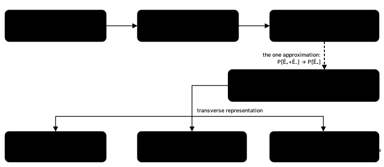
The chain of this primer. For a uniform medium, and once the scalar reduction is made, every step is exact except the dashed one, the unidirectional approximation. The three branches at the bottom are the transverse representations of Chapters 3–6.#
2.4 Self-steepening and space-time focusing are already there#
Older envelope equations add the optical shock (self-steepening) and space-time focusing as correction operators, \((1+\tfrac{i}{\omega_0}\partial_t)\) on the nonlinearity and its inverse on diffraction. In the UPPE they are not separate terms. They are the frequency dependence of the coefficients you have just met.
Self-steepening is the \(\omega\) in the numerator of the nonlinear coefficient. Write
\(\omega=\omega_0+(\omega-\omega_0)\). On an envelope, \((\omega-\omega_0)\to i\partial_t\), so
the coefficient becomes \(\frac{i\omega_0}{2\varepsilon_0cn}(1+\tfrac{i}{\omega_0}\partial_t)\)
acting on \(P\) (Kolesik and Moloney 2004, Eqs. 53 and 55). The familiar shock operator is
the first-order Taylor expansion of something the UPPE carries exactly. solprop’s
shock=False option freezes this numerator at the carrier, which removes self-steepening
and changes nothing else
(from polarisation to propagation).
Space-time focusing is the frequency dependence of diffraction. Expanding \(k_z\) for small \(k_\perp\) gives \(k_z\approx k-k_\perp^2/2k\), and the \(1/k\propto1/\omega\) means that higher frequencies diffract less. Expanding that \(1/\omega\) about the carrier gives the operator \((1+\tfrac{\omega-\omega_0}{\omega_0})^{-1}\) of the nonlinear envelope equation (Kolesik and Moloney 2004, Eq. 54). Truncating it at first order gives a diffraction that changes sign near \(2\omega_0\), which is unphysical (their Sec. VI D). solprop’s free-space routes use the exact square root, so there is nothing to truncate (Chapter 6).
The general lesson, repeated throughout the literature, is that every approximate envelope equation is the UPPE with its linear operator \(K\) or its coupling \(Q\) expanded about a reference frequency (Kolesik and Moloney 2004, Sec. VI). The expansions are where the approximations live. Keeping \(K\) and \(Q\) exact removes them.
2.5 Guided modes#
For a waveguide the transverse Fourier components are replaced by guided modes. Kolesik and Moloney (2004, Eq. 18) write the coupled-mode equation for the amplitude \(A_m(\omega,z)\) of mode \(m\) with transverse field \(\boldsymbol{\mathcal E}_m(\omega,x,y)\) as
written here in the frequency domain, with \(2N_m\) the Poynting-flux normalisation of the mode (their Eq. 12). Applied to plane waves, this equation reproduces the bulk UPPE. Applied to the modes of a fibre or capillary, it gives the modal UPPE that solprop’s waveguide routes solve. The nonlinear polarisation is computed from the field synthesised from all the modes and then projected back onto each one. Chapters 4 and 5 explain how solprop does that projection and how its modes are normalised. For now the point is structural: the waveguide equation is the same equation, with \(k_z\to\beta_m(\omega)\) and an overlap integral in place of a transverse Fourier transform.
2.6 The moving frame#
The pulse moves at roughly its group velocity, so in the laboratory frame it leaves any finite time window after a short distance. Every propagation code therefore uses a retarded time \(\tau=t-\beta_1z\), where \(\beta_1\) is an inverse velocity chosen by the code. When \(\beta_1\) changes along \(z\), as below, the frame is \(\tau=t-\int_0^z\beta_1(z')\,\mathrm dz'\), of which \(t-\beta_1z\) is the constant special case; the local subtraction is still \(\beta_1(z)\omega\). In the frequency domain the change of variable only subtracts a term linear in \(\omega\) from the propagation constant, \(k_z\to k_z-\beta_1\omega\), and leaves the coupling untouched (Couairon et al. 2011, Eqs. 15–18).
The frame is a coordinate, not physics. Couairon et al. (2011, after Eq. 186) note that the frame velocity “is an arbitrary parameter which does not reflect any physics”. Two things nevertheless make the choice matter in practice.
First, \(\beta_1\) should be the group delay at the reference frequency, so that the pulse stays near the centre of the window. solprop computes it from the effective index with an analytically differentiated \(\mathrm dn/\mathrm d\omega\),
and re-evaluates it at every \(z\), so that the window follows the pulse along a pressure gradient or a taper. A finite-difference derivative would have a roughness floor that limits the accuracy of everything built on it (from the effective index).
Second, a set of modes must share one frame. The nonlinear term multiplies the fields of different modes at the same instant. If each mode had its own frame, mode \(p\) would drift against mode 1 by \((\beta_{1,p}-\beta_{1,1})z\), and the code would be multiplying fields that were never simultaneous. That drift is the group-delay walk-off, and it is physics. For the \(\mathrm{HE}_{11}\) and \(\mathrm{HE}_{12}\) modes of a 125 µm capillary at 800 nm it is 43 fs per metre, and per-mode frames under-populate the higher modes of a four-mode resonant-dispersive-wave run by two to four orders of magnitude. solprop takes the frame from the first mode of the set (one frame for a mode set).
A related trick removes not only the group delay but also the carrier phase. On an envelope grid, subtracting the constant \(\beta_0=\beta(\omega_{\rm ref})\) stops the envelope rotating at \(\beta_0\) radians per metre. What remains of the propagation constant is \(\beta-\beta_0-\beta_1(\omega-\omega_{\rm ref})\), a few tens of inverse metres instead of the \(10^7\) m⁻¹ of \(\beta\) itself. A field grid cannot do this. Its stored object is the real field, and a constant phase on the half-spectrum of a real field rotates the carrier-envelope phase. That would change the field the third harmonic and tunnelling ionisation respond to. A field grid therefore keeps \(\beta_0\) and measures the frame term from zero frequency, \(\beta-\beta_1\omega\). An envelope grid that carries a third-harmonic term keeps \(\beta_0\) too, because the harmonic’s phase is tied to the true carrier phase (which terms the frame removes).
2.7 The envelope equation is the same equation#
Factor the carrier out of the field, \(\tilde E(\omega)\propto\tilde A(\Omega)\) with \(\Omega=\omega-\omega_0\), and the UPPE becomes an equation for the envelope spectrum:
(Couairon et al. 2011, Eqs. 38–40). This is the field equation with every frequency relabelled. No approximation has been made, provided that \(\mathcal K\) and \(\mathcal Q\) are evaluated exactly, rather than as Taylor series in \(\Omega\), and that the envelope of the polarisation keeps all the frequency content the field would have. Kolesik and Moloney (2014, Eq. 13) make the same point. Replacing the Taylor dispersion operator of the nonlinear envelope equation by the full \(k(\omega)-k_0-k_0'(\omega-\omega_0)\) removes the dispersion approximation entirely. That is precisely solprop’s envelope-grid operator.
The approximations of envelope models are therefore elsewhere:
The polarisation drops harmonics. An envelope model with only \(\tfrac34|A|^2A\) omits third-harmonic generation. solprop’s envelope grid can carry the harmonic term, with a \(e^{-2i\omega_0t}A^3\) piece, but only with enough oversampling to represent it (Chapter 8). Two separate envelopes for the fundamental and the harmonic become inconsistent once their spectra overlap (Couairon et al. 2011, end of §2.4.2), so solprop carries the harmonic on a single grid, never as a second envelope.
The responses are cycle-averaged. An exact complex envelope keeps the carrier phase and can reconstruct the real field, but a response model written in \(|A|^2\) alone knows only the cycle-averaged intensity. Tunnelling ionisation depends on the instantaneous field, so an envelope plasma model built that way has to average the rate over a cycle. solprop does this explicitly as a separate model (Chapter 10).
The coefficients are expanded. Taylor-expanding \(\mathcal K\) gives the familiar \(\beta_2,\beta_3,\dots\) dispersion operator, and Taylor-expanding \(\mathcal Q\) gives the shock term. Both are truncations, and the truncated \(\mathcal K\) has a finite radius of convergence (§1.3).
The reference frequency is, in the words of Kolesik and Moloney (2014, after Eq. 6), “arbitrarily chosen ‘gauge’ parameters”. An exact equation does not depend on it. An approximate one does, and Kolesik and Moloney (2004, Sec. VI G) suggest a useful test: repeat a run with a shifted reference frequency, and do not trust the parts of the spectrum that change. In solprop the reference frequency also fixes the frame, so the test also checks that the window was wide enough.
2.8 Exact linear propagation: the interaction picture#
The linear part of the UPPE is diagonal in frequency (and in mode, for independent modes), so it can be integrated exactly. Write \(\tilde E=A\,e^{ik_zz}\). The linear term disappears and only the nonlinear source remains, rotated by the linear phase:
(Kolesik and Moloney 2014, Eqs. 27–28). In their words, “the integration step is controlled solely by the strength of the nonlinear wavepacket reshaping, and it can be arbitrary long in the linear case”. The linear phase can become enormous, so practical codes re-anchor it at the start of every step: after each step, \(A\) is multiplied by the phase accumulated over that step and the origin is moved (Couairon et al. 2011, Eq. 182).
When the guide varies along \(z\), because of a pressure gradient or a taper, the propagation constant depends on \(z\) and the accumulated phase is an integral, \(\Phi(\omega,z)=\int_0^zD(\omega,z')\,\mathrm dz'\). solprop computes that integral to a controlled tolerance instead of evaluating the operator at one point per step. A right-endpoint rule would be first-order accurate in the step, and the adaptive error estimate cannot see that error (Chapter 12). This interaction picture, and the integrators built on it, are the subject of Chapter 12.
2.9 The equation solprop solves#
Everything above can now be assembled. For a mode \(m\) (or a transverse Fourier component in free space), solprop propagates a spectral amplitude \(\tilde a_m(\omega,z)\) obeying, in the optics convention of this primer,
with \(\beta_m=(\omega/c)\operatorname{Re}n_{{\rm eff},m}\) and \(\alpha_m=(2\omega/c)\operatorname{Im}n_{{\rm eff},m}\). The pieces are:
The bracket is the linear operator \(D_m\). It holds the full dispersion and loss of the mode in the co-moving frame of §2.6. On a field grid \(\beta_0\) is kept and the frame term is \(\beta_1\omega\); an envelope grid with a third-harmonic term also keeps \(\beta_0\). \(\alpha_{\rm abs}(\omega)\) is the spectral absorbing collar, expressed as a rate (Chapter 11). The \(-\tfrac12\partial_z\ln w_m\) term, with \(w_m=\operatorname{Re}n_{{\rm eff},m}\), keeps the energy of the true-power amplitude correct where \(w\) varies along \(z\). It vanishes for a uniform guide and on the GNLSE route (Chapter 4).
The nonlinear term \(N_m\) is the transformed polarisation (including currents) multiplied by
\[ +\frac{i\omega}{2\varepsilon_0c\operatorname{Re}n_{{\rm eff},m}(\omega)} \]and projected onto mode \(m\). In free space the corresponding factor is \(i\omega^2/(2\varepsilon_0c^2\operatorname{Re}k_z)\) (Chapter 6).
The mode part of the operator and the prefactor are zero outside the active band, \(\omega_{\min}/2<\omega<1.1\,\omega_{\max}\), where \(\omega_{\min}\) and \(\omega_{\max}\) are the limits of the grid you asked for. Outside that band the effective index may have no meaning, for example at zero frequency on a field grid. The prefactor is zero there rather than one, so that no unnormalised polarisation remains in the array. The spectral absorber \(\alpha_{\rm abs}\), by contrast, acts over the whole axis (where the operator is evaluated).
In the internal convention every \(+i\) above becomes \(-i\), which is how the linear operator and the solver pages write it.
One detail departs from the literal coefficient of §2.3. Kolesik’s \(k_z\) is complex in a lossy medium, but solprop uses only the real part of the index in the prefactor. The loss is carried once, in the linear operator. This is a modelling choice. Its effect is of relative order \(\operatorname{Im}n_{\rm eff}/\operatorname{Re}n_{\rm eff}\), which is negligible for any mode worth propagating. Ferrando et al. (2005, after Eq. 4) make the same choice in their modal forward-backward equations, for a different reason: to keep the transverse operator self-adjoint.
What to remember
For a uniform medium or guide, the scalar second-order wave equation splits exactly into a forward and a backward first-order equation. The single approximation that remains is to evaluate the polarisation from the forward field, \(\tilde P[\tilde E_++\tilde E_-]\to\tilde P[\tilde E_+]\).
Its error is of order \(10^{-4}\) in typical gas filaments and \(10^{-2}\) in tightly collapsing solids (illustrative estimates, not bounds). It fails at reflecting structures, at wavelength-scale gradients and for terahertz emission, none of which solprop models.
The scalar UPPE is \(\partial_z\tilde E=ik_z\tilde E+\frac{i\omega^2}{2\varepsilon_0c^2k_z}\tilde P-\frac{\omega}{2\varepsilon_0c^2k_z}\tilde J\) (Kolesik and Moloney 2004, Eq. 28). For a mode the coefficient is \(i\omega/(2\varepsilon_0cn)\).
Self-steepening is the \(\omega\) in the numerator. Space-time focusing is the \(\omega\) in diffraction. Approximate envelope equations are the UPPE with these expanded.
The moving frame is a coordinate, but a mode set must share one, because walk-off is physics. A field grid, and an envelope grid with a third-harmonic term, keep \(\beta_0\); an envelope grid without one removes it.
An envelope equation is exact if its operator and coupling are exact and its polarisation keeps every frequency the field would have.
solprop uses \(\operatorname{Re}n_{\rm eff}\) in the prefactor and zeros the mode operator and the prefactor outside the active band; the absorber acts everywhere.
The precise statements are in the linear operator, from polarisation to propagation and the algorithms. Chapter 3 collapses the transverse dimension to a single number and arrives at the generalised nonlinear Schrödinger equation.