10. Ionisation, plasma and noise#
At the intensities of soliton self-compression and filamentation, typically \(10^{13}\) to \(10^{14}\) W/cm², a laser field is strong enough to free electrons from atoms and molecules within a single pulse. The freed electrons are a plasma. The negative change it makes to the refractive index defocuses the beam and shifts the spectrum towards the blue, and the energy spent freeing the electrons is lost from the pulse. Ionisation is also the response that departs most from everything in the previous chapters. It is not a power series in the field. It depends on the instantaneous field in a steeply nonlinear way, and it has memory, because electrons once freed stay free for the duration of the pulse.
This chapter covers how solprop models these effects. It starts with the strong-field physics that sets the rate, then shows how the rate becomes a population, and the population becomes the two currents of Geissler et al. (1999). It explains why the integrals must be computed with care, how the envelope route averages over a cycle, and what the shot noise that seeds many of these processes is. A last section points to the time-dependent Schrödinger response for when rates are not enough.
10.1 Multiphoton, tunnelling and in between#
An atom with ionisation potential \(I_p\) in a field of amplitude \(E\) and frequency \(\omega\) can be ionised in two limiting ways. At low intensity or high frequency, it absorbs several photons at once, and the rate scales as \(I^K\), with \(K\) the number of photons needed. At high intensity or low frequency, the field bends the Coulomb potential enough for the electron to tunnel through the barrier within an optical half-cycle. The rate then depends exponentially on \(1/E\). Keldysh (1965, Eq. 17) showed that one parameter separates the two:
the tunnelling time multiplied by the angular frequency, that is, \(2\pi\) times its ratio to the optical period. \(\gamma\gg1\) is multiphoton and \(\gamma\ll1\) is tunnelling. For argon at 800 nm and \(10^{14}\) W/cm², \(\gamma\approx1.15\). Filaments and the pulses inside gas-filled fibres usually sit in this intermediate regime, where neither limit holds. That is why the theory of Perelomov, Popov and Terent’ev (1966), which bridges the two, is the basis of solprop’s default rates. At still higher fields the barrier is suppressed altogether. This happens above \(E_b=I_p^2/4Z\) in atomic units, \(4.3\times10^{10}\) V/m or about \(2.5\times10^{14}\) W/cm² for argon (Tong and Lin 2005, Eq. 1).
10.2 The rate#
solprop takes its ionisation rates from optmat (rates from optmat). For the atoms, the recommended model is the short-range rate of Perelomov, Popov and Terent’ev (1966, Eq. 54), with its Keldysh functions \(g(\gamma)\) and \(A_m\) (their Eqs. 33 and 55). It is multiplied by a Coulomb correction. Its static part, \((2F_0/F)^{2n^*}\) in atomic units with \(F_0=(2I_p)^{3/2}\) and \(n^*=Z/\sqrt{2I_p}\), is the one Perelomov and Popov (1967, Eq. 42) showed “has the same form as for a static field”, with no dependence on \(\gamma\). optmat multiplies it by an empirical frequency-dependent factor, \((1+2\gamma/e)^{-2n^*cs}\) with \(s=n^*\omega/2I_p\) and \(c=5.25\), which it fitted to one-electron time-dependent Schrödinger calculations. The model with the static factor alone remains available for comparison. The common Ilkov form (Ilkov, Decker and Chin 1992, Eq. 8), used in many propagation codes, writes the Coulomb factor and the Keldysh prefactor under one bracket with \(\sqrt{1+\gamma^2}\), and that is not the same thing. At the highest fields, the rate is multiplied by the empirical barrier-suppression correction of Tong and Lin (2005, Eq. 2), \(\exp[-\alpha(Z^2/I_p)(F/\kappa^3)]\), with their fitted \(\alpha\). For the molecules, optmat supplies molecular models with orientation-averaged structure factors.
In the static limit, the cycle-averaged form of these rates is the familiar ADK rate (Ammosov, Delone and Krainov 1986, Eq. 1), whose factor \((3F/\pi F_0)^{1/2}\) is the average of the instantaneous tunnelling rate over a cycle. That factor marks the essential distinction for a propagation code. A cycle-averaged rate is a function of the envelope’s amplitude. An instantaneous rate is a function of the field at each moment. A field-grid calculation needs the instantaneous rate, since it resolves the cycle itself. An envelope calculation needs the cycle average. optmat provides both, consistent with each other: averaging the instantaneous rate over a cycle reproduces the cycle-averaged one to 1.5% at 800 nm. Obtaining an instantaneous rate by dividing a cycle-averaged one by the tunnelling-limit factor overestimates the ionisation of argon (with the Ilkov form of the rate) by 11% at 800 nm and \(10^{14}\) W/cm², and by 85% at 400 nm and \(2\times10^{13}\) W/cm².
Three practical features complete the rate as solprop uses it (thresholds, ceilings and why both exist):
A threshold. Below a field where the rate falls under \(10^{-30}\) s⁻¹ it is exactly zero. As §10.3 shows, the loss current divides by the field, and an exact zero keeps it finite.
A ceiling. The rate is capped at one event per atomic unit of time, \(4.1\times10^{16}\) s⁻¹, and held constant above a maximum field, typically twice the barrier-suppression field. These models are not valid there, and the hold is recorded.
A table. The rate is tabulated on knots uniform in \(\log E\), refined to a relative accuracy of \(10^{-6}\).
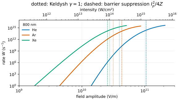
optmat’s recommended instantaneous rates for three noble gases at 800 nm, from their
thresholds to their maximum fields, with the Keldysh parameter equal to one (dotted) and the
barrier-suppression field (dashed) marked for each. Computed with solprop’s OptmatRate by
docs/primer/figures/primer_figures.py.#
optmat states an uncertainty factor for each rate at 800 nm: ×1.3 for helium, ×1.5 for neon and argon, up to ×3 for xenon. That is the accuracy of the physics. A rate wrong by a factor of 1.5 at an intensity where it scales as the eighth power corresponds to an intensity error of only 5%, which is one reason clamping is robust and also why it is hard to measure a rate from a propagation experiment.
10.3 The population and the two currents#
The fraction \(f\) of atoms ionised obeys
with \(f_0\) any pre-ionised fraction. This is the only form that both satisfies the population equation and stays bounded by one. The freed electrons affect the field through two currents (two currents), following Geissler et al. (1999, Eq. 4):
with \(n_e=\rho f\) the electron density. The free-electron current is the acceleration of electrons born at rest. For a fixed density it is exactly the Drude response, \(P=-\varepsilon_0(\omega_p^2/\omega^2)E\), with plasma frequency \(\omega_p^2=n_ee^2/(\varepsilon_0m_e)\). Its effect is a negative contribution to the refractive index, \(\Delta n\approx-n_e/(2\rho_c)\), where \(\rho_c=\varepsilon_0m_e\omega^2/e^2\) is the critical density, \(1.7\times10^{21}\) cm⁻³ at 800 nm (Couairon and Mysyrowicz 2007, Eq. 8). Geissler et al. call this term the one that “introduces predominantly phase effects, such as blueshifting”. A density rising in time shifts the instantaneous frequency up, and a density peaked on axis defocuses the beam. The loss current removes exactly the binding energy of each new electron: \(\mathbf E\cdot\mathbf J_{\rm loss}=I_p\rho\,\partial_tf\). Geissler et al. call it “a pure loss term”. solprop’s vector form, directed along the instantaneous field, is its own isotropic extension of Geissler et al.’s scalar equation, and the guide says so. The model is collisionless and has single ionisation only.
The currents enter the UPPE as equivalent polarisations, \(\tilde P=i\tilde J/\omega\) in the optics convention (Chapter 2), multiplied by the same prefactor as every other response. Two remarks follow. The loss current divides by the field, which is finite only because the rate is exactly zero where the field crosses zero. And because the currents are computed from the field at each node, a resolved mode set or a spatial grid sees the plasma where it actually forms, on axis. A mode-averaged calculation sees it at the effective-area intensity, 57% of the axial value (Chapter 5).
10.4 Integrating accurately#
The production source uses two running integrals in time: of \(W\) for the population and of \(n_eE\) for the free
current. It holds the residual current through the temporal collar and converts the two collared current
streams to an equivalent polarisation in frequency
(holding the post-pulse current).
The physical polarisation returned by PlasmaResponse.evaluate adds a third running integral, of
\(\mathbf J\). In the frequency domain, integration multiplies by
\(i/\omega\). The cumulative trapezoid rule multiplies by that factor times \(\rho(\theta)=(\theta/2)\cot(\theta/2)\),
with \(\theta=\omega\delta t\). On solprop’s default grid, the top of the active band is at \(\theta=1.15\). There a
trapezoid integral is 11% short, and the physical polarisation’s Drude double integral is 21% short.
The production held source has one trapezoid multiplier in its interior Drude response; its spectral
division does not add a second one. Collar and finite-window errors are separate
(how the current integrals are formed).
These errors sit at the blue edge of the spectrum, which is exactly where ionisation-induced blueshifts and
deep-ultraviolet dispersive waves live.
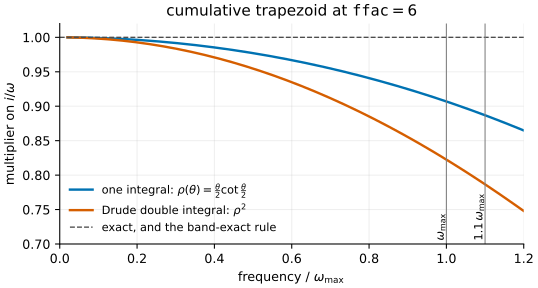
The cumulative trapezoid’s error as a spectral multiplier on a default field grid. Both the
single integral and the physical polarisation’s Drude double integral fall short towards the top of the band.
The production held source uses the single-integral curve away from the collar. The
band-exact rule holds each integral’s multiplier at one to \(10^{-5}\). Computed in closed form by
docs/primer/figures/primer_figures.py.#
solprop’s default integrates with a short symmetric filter applied before the trapezoid, designed so that the
combined response is exact to \(10^{-5}\) across the band. It uses nine taps by default and needs an oversampling
factor of at least about 3.55. The plain trapezoid remains available as an option. The \(10^{-5}\) describes the filter’s
multiplier for components inside its design band, not the total error of the plasma
polarisation, the ionisation or the work it does. Unresolved integrands, truncation at the ends of
the window, an undershoot of the filtered rate beside a sharp spike, a small mismatch between the
work and the population, and a look-ahead of a few samples all remain. A run records
plasma_undershoot, plasma_work_defect and plasma_boundary_level at each save plane for
inspection; they are not used as pass/fail conditions, and temporal refinement remains the check
(how the current integrals are formed).
This is an example of a
general principle in solprop’s numerics: an error that is the same at every step, of the representation
rather than of the step, cannot be found by refining the step, so it has to be designed out.
10.5 Plasma on an envelope#
An envelope grid does not resolve the optical cycle, so it cannot evaluate an instantaneous rate. solprop’s envelope plasma model averages over one frozen cycle (envelope plasma). At each time sample the envelope \(\mathbf a\) is held fixed, the real field \(\mathbf E_\theta=\operatorname{Re}(\mathbf ae^{-i\theta})\) is traced around a cycle, and the rate and the fundamental of the loss current are averaged:
with \(s\) the surviving neutral fraction. For elliptical light the average needs two separate angular moments of the rate. A single scalar loss coefficient gets the work right and the direction wrong, by 18% in one of the guide’s test cases. The Drude current becomes a first-order equation for its envelope. Its conversion to a polarisation uses the absolute optical frequency, \(\hat{\mathbf p}_D=-\hat{\mathbf d}_D/\omega^2\), not the detuning, which would introduce a false singularity at the carrier.
This model has limits that no resolution can remove. It assumes that the envelope, the ellipse and the neutral fraction change little over a cycle, and that depletion within one cycle is small. A long pulse can still ionise too quickly for that. In one strongly depleting short-pulse test the loss current is off by 22–27% despite accurate angular integration. Envelope plasma also cannot be combined with an envelope third harmonic. When the cycle matters, use a field grid.
10.6 When rates are not enough#
Rate models describe ionisation as a population process. They omit the response of electrons that are partly freed, their coherent contribution to harmonics, and the field dependence of the bound response beyond the cubic. For helium, solprop can replace its Kerr and plasma responses together by the current of a time-dependent Schrödinger equation, solved at each radial node by Pyroraptor, a separate optional package that is not yet publicly available (TDSE response in a helium capillary). The source is the part of that current beyond linear response, since the linear part is already in the refractive index. Two atomic models are offered:
A single active electron in a model potential. One electron stands in for two, so the current is scaled by an empirical factor of 1.537, chosen by calibration.
haCC, a correlated two-electron model: a two-electron neutral near the nucleus coupled to channels of a frozen He⁺ ion and one active electron. haCC(1) keeps the 1s ion only. haCC(5) adds the four \(n=2\) ionic states and so part of the core’s polarisation (two atomic models). Its current already sums both electrons, so the scale is exactly one and nothing is calibrated. The difference between haCC(1) and haCC(5) measures sensitivity to the excited ion, not the full truncation error. A fast variant with a lower spectral cut and a larger time step needs 2.3 times fewer steps for the same model.
Each source evaluation drives fresh atoms with the local field over a finite atomic window, and atoms ionised by a strong pulse are still drifting when the window ends. Switching their current off there would radiate a spurious near-infrared signal. The source is therefore formed from the gated time derivative of the current, which has no such edge, divided by \(i\omega\) (the edge-free gated source). What the window cannot remove is the current after it closes. At the default 60 fs it leaves a sensitivity of a few per cent in the source above about 900 nm.
Both models are research configurations. haCC propagation is demonstrated over one segment of a capillary, not qualified against an exact solution or over a full run, and each source evaluation takes minutes on a many-core node. Neither should be treated as a qualified replacement for the rate models.
10.7 Shot noise#
Many of the processes in this primer grow from noise: modulational instability, the incoherent part of a supercontinuum, Raman scattering from the vacuum. A deterministic simulation needs a seed. solprop adds one photon of energy per spectral bin, with a random phase and a deterministic modulus, on the active band of both grids (one photon per bin):
This is the semiclassical seed of the supercontinuum literature. It is not a quantum-state model. In the truncated-Wigner treatment of Drummond and Corney (2001, Eq. 6.13), the vacuum is half a photon per mode, with a Gaussian random amplitude as well as a random phase, and results must be corrected for operator ordering. Raman scattering adds its own thermal and vacuum Langevin noise there (their Eq. 6.16), which solprop does not. solprop’s second, “modified” model re-injects the same noise realisation into the nonlinear step at every \(z\). It advances the realisation by the phase of the linear operator only (dispersion, but no gain or loss), so that it stays in step with the field it seeds, at the price of about eight times as many steps. Ensembles of runs with different seeds give spectral coherence and fluctuation statistics (processing).
What to remember
Keldysh’s \(\gamma=\omega\sqrt{2m_eI_p}/eE\) separates multiphoton (\(\gamma\gg1\)) from tunnelling (\(\gamma\ll1\)). Most gas-fibre and filament physics sits near \(\gamma\approx1\), which is why PPT is the default.
The rates come from optmat: PPT with a Coulomb factor and the Tong–Lin correction for atoms, molecular models otherwise, each with an uncertainty factor. The Coulomb factor is Perelomov and Popov’s static one times an empirical frequency-dependent correction. A field grid needs the instantaneous rate, an envelope the cycle average. Do not convert one to the other by the tunnelling factor.
\(f=1-(1-f_0)e^{-\int W}\). The free current is Drude, and gives blueshift and defocusing. The loss current removes \(I_p\) per electron and divides by the field, which the exact-zero threshold makes safe.
Trapezoid integration is 11% (single) and 21% (Drude) short at the top of the band. solprop’s band-exact filter removes that error.
The envelope plasma averages a frozen cycle with two ellipse moments. It fails when one cycle depletes the gas, and cannot be combined with an envelope harmonic.
For helium, a TDSE current from Pyroraptor can replace Kerr and plasma together: a single active electron scaled by a calibrated 1.537, or the two-electron haCC(1)/haCC(5) at scale one. Both are research configurations.
The noise seed is one photon per bin with random phase: semiclassical, not a Wigner vacuum, and with no Raman Langevin noise.
The precise statements are in strong-field ionisation, carrier-resolved plasma, envelope plasma and shot noise. Chapter 11 begins the numerical part of the primer.